rizer.io.radiation_data_reader#
Classes#
Load and process the radiation data for a gas, assuming LTE. |
Module Contents#
- class rizer.io.radiation_data_reader.RadiationDataReader(gas_name: str, pressure_atm: int, emission_radius_mm: int, source: str)#
Load and process the radiation data for a gas, assuming LTE.
LTE (Local Thermodynamic Equilibrium) means that thermal and chemical equilibrium are established. The data is assumed to be given at a fixed pressure.
Methods are provided to interpolate the data and plot it. The interpolations are linear, and out-of-bounds values take the value at the boundary.
- Parameters:
gas_name (
str) – Gas used for the radiation data.pressure_atm (
int) – Pressure (in atm) for the radiation data.emission_radius_mm (
int) – Emission radius (in mm) for the radiation data. The net emission coefficient depends on the size of the emitting volume.source (
str) – Source used for the radiation data.
Examples
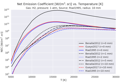
Plot radiation data vs. temperature for CH4, H2 and N2.
Plot radiation data vs. temperature for CH4, H2 and N2.- temperature#
- nec_data#
- load_data() tuple[numpy.ndarray, numpy.ndarray]#
Load the data from the files.
Files are expected to be in ./data/LTE_radiation.
The radiation data file is expected to be a CSV file with the following columns:
Temperature [K]
Net emission coefficient [W/(m^3.sr)]
It is assumed that the data is sorted by increasing temperature. It is also assumed that the header is 3 lines long.
- Returns:
Tuple containing the following arrays:
temperature: Temperature [K]
nec: Net emission coefficient [W/(m^3.sr)]
- Return type:
- plot(x: str = 'temperature', y: str = 'net_emission_coefficient', show: bool = True, yscale: str = 'linear', fig_ax: tuple[matplotlib.figure.Figure, matplotlib.axes.Axes] | None = None, **plot_options) tuple[matplotlib.figure.Figure, matplotlib.axes.Axes]#
Plot data.
- Parameters:
x (
str) – X axis data. Can only be “temperature” or “T”.y (
str) – Y axis data. Could be “nec” or “net_emission_coefficient”. Can also be “temperature” or “T”, but that would be a trivial plot.show (
bool, optional) – Whether to display the plot immediately (default is True).yscale (
str, optional) – The scale of the y-axis. Options are “linear” or “log” (default is “linear”).fig_ax (
tupleofmatplotlib.figure.Figure,matplotlib.axes.AxesorNone, optional) – A tuple containing a Matplotlib Figure and Axes to plot on. If None, a new figure and axes are created (default is None).**plot_options – Additional keyword arguments to pass to the plotting function. E.g., label, color, linestyle, marker, etc.
- Returns:
The figure and axes objects of the plot.
- Return type:
- Raises:
ValueError – If an invalid variable is specified for the x or y axis.
Examples
>>> from rizer.io.radiation_data_reader import RadiationDataReader
>>> # Define the hydrogen data.
>>> hydrogen_data = RadiationDataReader(
...     gas_name="H2",
...     pressure_atm=1,
...     emission_radius_mm=0,
...     source="Gueye2017",
... )
>>> # Plot the data.
>>> fig, ax = hydrogen_data.plot(x="temperature", y="nec", show=False)