rizer.thermal_plasma.elenbaas_heller#

Attributes#

H2_lte_data

Classes#

ElenbaasHeller

Elenbaas-Heller model for the electrical conductivity of a gas mixture.

Module Contents#

Elenbaas-Heller model for the electrical conductivity of a gas mixture.

Parameters:

R (float | int) – Outer radius, in m.
electric_field (None | float | int, optional) – Electric field, in V/m.
current (None | float | int, optional) – Current, in A, by default None.
data (FitLTEData) – LTE data for the gas mixture.
nb_points (int, optional) – Number of points for the radial distance, by default 1000.

Notes

The Elenbaas-Heller equation is given by (see [Elenbaas1951]):

\[\frac{1}{r} \frac{d}{dr} \left( r \kappa(T) \frac{dT}{dr} \right) + \sigma(T) E^2 + P^{rad}(T)= 0\]

where:

\(r\) is the radial distance,
\(\kappa(T)\) is the thermal conductivity,
\(T\) is the temperature,
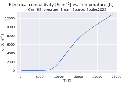
\(\sigma(T)\) is the electrical conductivity,
\(E\) is the electric field,
\(P^{rad}(T)\) is the radiative power.

Neglecting the radiative power, the Elenbaas-Heller equation becomes:

\[\frac{1}{r} \frac{d}{dr} \left( r \kappa(T) \frac{dT}{dr} \right) + \sigma(T) E^2 = 0\]

Introducing \(\Theta(T) = \int_0^T \kappa(s) ds\), the Elenbaas-Heller equation becomes:

\[\frac{1}{r} \frac{d}{dr} \left( r \frac{d\Theta}{dr} \right) + \sigma(\Theta) E^2 = 0\]

Making some approximations (see [Gueye2017]), the expression for the electrical conductivity can be written as:

\[\begin{split}\sigma(\Theta) = \begin{cases} 0 & \text{if } \Theta < \theta_\sigma (r \in ]r_0, R])\\ a_\sigma (\Theta - \theta_\sigma) & \text{if } \Theta \geq \theta_\sigma (r \in [0, r_0]) \end{cases}\end{split}\]

where:

\(a_\sigma\) is the slope of the electrical conductivity vs. integrated thermal conductivity, in (S/m)/(W.m^-1),
\(\theta_\sigma\) is the first value of the integrated thermal conductivity where the electrical conductivity is non-zero, in W/m,
\(r_0\) is the inner (arc) radius, in m, such that radius lower than \(r_0\) corresponds to non-zero electrical conductivity, and radius greater than \(r_0\) corresponds to zero electrical conductivity,
\(R\) is the outer (torch) radius, in m.

With the following boundary conditions:

Assuming the wall is maintened at 0 K, \(\Theta(r=R) = \int_0^{T(R)=T_w=0} \kappa(s) ds = 0\).
By symmetry, \(\frac{d\Theta}{dr}(r=0) = \left( \frac{dT}{dr} \lambda(T) \right)(r=0) = 0\).
By continuity, \(\Theta(r_0^-) = \Theta(r_0^+) = \theta_\sigma\).
And by continuity of the derivative, \(\frac{d\Theta}{dr}(r_0^-) = \frac{d\Theta}{dr}(r_0^+)\).

The analytical solution to the Elenbaas-Heller equation is then given by:

\[\begin{split}\Theta(r) = \begin{cases} \theta_\sigma \left( 1 + \frac{J_0(\epsilon r)}{J_1(\epsilon r_0)} \frac{1}{r_0 \epsilon \ln(R/r_0)} \right) & \text{if } r \in [0, r_0]\\ \theta_\sigma \frac{\ln(r/R)}{\ln(r_0/R)} & \text{if } r \in ]r_0, R] \end{cases}\end{split}\]

where:

\(\epsilon = \sqrt{a_\sigma E^2}\),
\(J_0\) is the Bessel function of the first kind of order 0,
\(J_1\) is the Bessel function of the first kind of order 1.

Examples

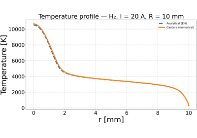
Elenbaas-Heller model for H₂ DC plasma.

gas_data#

a_sigma#

theta_sigma#

temperature#

theta#

analytical_theta_vs_radius(r: float) → float#

Analytical solution to the Elenbaas-Heller equation.

Parameters:: r (float) – Radial distance.
Returns:: Integrated thermal conductivity at radial distance r.
Return type:: float
Raises:: ValueError – If r is not between 0 and R.

Notes

The analytical solution to the Elenbaas-Heller equation is given by:

\[\begin{split}\Theta(r) = \begin{cases} \theta_\sigma \left( 1 + \frac{J_0(\epsilon r)}{J_1(\epsilon r_0)} \frac{1}{r_0 \epsilon \ln(R/r_0)} \right) & \text{if } r \in [0, r_0]\\ \theta_\sigma \frac{\ln(r/R)}{\ln(r_0/R)} & \text{if } r \in ]r_0, R] \end{cases}\end{split}\]

where:

\(\epsilon = \sqrt{a E^2}\), with \(a\) the constant, slope of the electrical conductivity \(\sigma\) vs. integrated thermal conductivity \(\Theta\), and \(E\) the electric field,
\(\theta_\sigma\) is the constant, initial value of the thermal conductivity,
\(J_0\) is the Bessel function of the first kind of order 0,
\(J_1\) is the Bessel function of the first kind of order 1,
\(r_0\) is the inner radius, which should be such that \(r_0 \sqrt{a E^2}\) is a zero of the Bessel function \(J_0\),
\(R\) is the outer radius.

get_inner_radius(nth_zero: int = 0) → float#

Get the inner radius.

Parameters:: nth_zero (int, optional) – Nth zero of the Bessel function \(J_0\), by default 0.
Returns:: Inner radius.
Return type:: float

Notes

The inner radius is such that \(r_0 \sqrt{a_\sigma E^2}\) is a zero of the Bessel function \(J_0\).

analytical_current() → float#

Calculate the current.

Returns:: Current.
Return type:: float

Notes

The current is given by:

\[I = \frac{2 \pi \theta_\sigma}{E \ln(R/r_0)}\]

where:

\(\theta_\sigma\) is the constant, initial value of the thermal conductivity,
\(E\) is the electric field,
\(R\) is the outer radius,
\(r_0\) is the inner radius, such that \(r_0 \sqrt{a E^2}\) is a zero of the Bessel function \(J_0\).

get_electric_field_vs_current(target_current: float, initial_electric_field: float = 1000.0) → float#

Get the electric field.

Parameters:

target_current (float) – Target current.
initial_electric_field (float, optional) – Initial electric field for the solver, by default 1000.0 V/m.

Returns:

Electric field.

Return type:

float

Notes

The electric field is such that the analytical current is equal to the target current.

get_temperature_vs_radius(r: float, initial_temperature: float = 300.0) → float#

Get the temperature at a given radial distance.

Parameters:

r (float) – Radial distance.
initial_temperature (float, optional) – Initial temperature for the solver, by default 300.0 K.

Returns:

Temperature.

Return type:

float

Notes

The temperature is such that the integrated thermal conductivity is equal to the integrated thermal conductivity at the radial distance r.

The integrated thermal conductivity is given by:

\[\Theta(T(r)) = \int_0^{T(r)} \kappa(s) ds\]

where:

\(\kappa\) is the thermal conductivity,
\(T\) is the temperature.

compute_radiative_power_density_at_r(r: float) → float#

Compute the radiative power density at a given radial distance.

Parameters:: r (float) – Radial distance.
Returns:: Radiative power density.
Return type:: float

Notes

The radiative power density is given by (see equation 13 in [Gueye2017]):

\[P^{rad} = \vec{\nabla} \cdot \vec{q^{rad}} = 4 \pi \text{NEC}\]

where:

\(\text{NEC}\) is the net emission coefficient.

compare_power_density(r: float) → tuple[float, float, float]#

Compare the power density.

Parameters:: r (float) – Radial distance.
Returns:: Joule power density, conductive power density, radiative power density.
Return type:: tuple[float, float, float]

Notes

The power density is given by:

\[P = \sigma E^2 + \frac{1}{r} \frac{d}{dr} \left( r \frac{d\Theta}{dr} \right) + P^{rad}\]

where:

\(\sigma E^2\) is the Joule power density,
\(\frac{1}{r} \frac{d}{dr} \left(r \frac{d\Theta}{dr} \right)\) is the conductive power density,
\(P^{rad}\) is the radiative power density.
\(\sigma\) is the electrical conductivity,
\(E\) is the electric field.
\(\Theta = \int_0^T \kappa(s) ds\) is the integrated thermal conductivity, with \(\kappa\) the thermal conductivity and \(T\) the temperature.