rizer.io.thermo_transport_data_reader#
Classes#
Load and process the thermodynamic and transport data for a gas, assuming LTE. |
Module Contents#
- class rizer.io.thermo_transport_data_reader.ThermoTransportDataReader(gas_name: str, pressure_atm: int, source: str, ignore_missing_values: bool = False)#
Load and process the thermodynamic and transport data for a gas, assuming LTE.
LTE (Local Thermodynamic Equilibrium) means that thermal and chemical equilibrium are established. The data is assumed to be given at a fixed pressure.
Methods are provided to interpolate the data and plot it. The interpolations are linear, and out-of-bounds values take the value at the boundary.
- Parameters:
Examples

Computing and comparing the properties of an CH_4 plasma.
Computing and comparing the properties of an CH_4 plasma.
Example: Calculating the properties of an CH_4 plasma.
Example: Calculating the properties of an CH_4 plasma.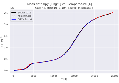
Plot thermodynamic properties of H₂ vs. temperatures.
Plot thermodynamic properties of H₂ vs. temperatures.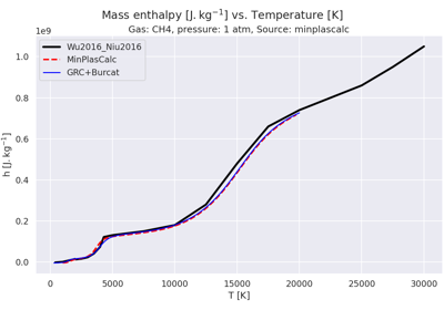
Plot thermodynamic properties of CH₄ vs. temperatures.
Plot thermodynamic properties of CH₄ vs. temperatures.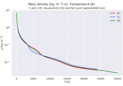
Plot thermodynamic and transport data vs. temperature for a plasma of Air, O2 or N2 in LTE.
Plot thermodynamic and transport data vs. temperature for a plasma of Air, O2 or N2 in LTE.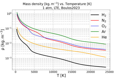
Plot thermodynamic and transport data vs. temperature for a plasma of H2, O2, N2, Ar, He in LTE.
Plot thermodynamic and transport data vs. temperature for a plasma of H2, O2, N2, Ar, He in LTE.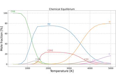
Compare thermal conductivity vs. temperature for a plasma of methane.
Compare thermal conductivity vs. temperature for a plasma of methane.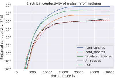
Plot electrical conductivity vs. temperature for a plasma of methane.
Plot electrical conductivity vs. temperature for a plasma of methane.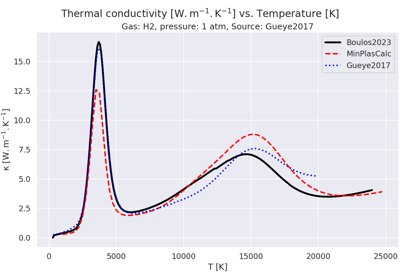
Plot transport data vs. temperature for a plasma of hydrogen.
Plot transport data vs. temperature for a plasma of hydrogen.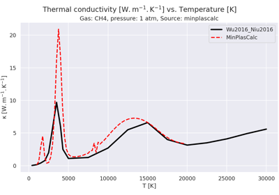
Plot transport data vs. temperature for a plasma of methane.
Plot transport data vs. temperature for a plasma of methane.- ignore_missing_values = False#
- temperature#
- density#
- enthalpy#
- heat_capacity_constant_pressure#
- dynamic_viscosity#
- thermal_conductivity#
- electrical_conductivity#
- thermal_diffusivity#
- theta#
- load_data() tuple[numpy.ndarray, numpy.ndarray, numpy.ndarray, numpy.ndarray, numpy.ndarray, numpy.ndarray, numpy.ndarray]#
Load the data from the files.
Files are expected to be in ./data/LTE_thermo_transport.
The thermo/transport data file is expected to be a CSV file with the following columns:
Temperature [K]
Density [kg/m3]
Enthalpy [J/kg]
Specific heat [J/kg.K]
Viscosity [kg/m.s]
Thermal conductivity [W/m.K]
Electrical conductivity [S/m]
It is assumed that the data is sorted by increasing temperature. It is also assumed that the header is 3 lines long.
- Returns:
Tuple containing the following arrays:
temperature: Temperature [K]
density: Density [kg/m3]
enthalpy: Enthalpy [J/kg]
cp: Specific heat at constant pressure [J/kg.K]
dynamic_viscosity: Viscosity [kg/m.s]
thermal_conductivity: Thermal conductivity [W/m.K]
electrical_conductivity: Electrical conductivity [S/m]
- Return type:
- compute_theta() numpy.ndarray#
Compute the integrated thermal conductivity.
Notes
The integrated thermal conductivity is defined as:
\[\theta(T) = \int_{T_0}^{T} \kappa(T') dT'\]where \(T_0\) is the first temperature value available in the dataset. By convention, \(theta(T_0) = 0\).
It is computed using the trapezoidal rule.
- alpha(T: float) float#
Get the thermal diffusivity at a given temperature.
- Parameters:
T (
float) – Temperature [K].- Returns:
Thermal diffusivity [m^2/s] at the given temperature.
- Return type:
Notes
The thermal diffusivity is computed as:
\[\alpha = \frac{\kappa}{\rho c_p}\]where:
\(\kappa\) is the thermal conductivity [W/(m.K)]
\(\rho\) is the density [kg/m^3]
\(c_p\) is the heat capacity at constant pressure [J/(kg.K)]
- plot(x: str, y: str, show: bool = True, yscale: str = 'linear', fig_ax: tuple[matplotlib.figure.Figure, matplotlib.axes.Axes] | None = None, ax_title: str | None = None, **plot_options) tuple[matplotlib.figure.Figure, matplotlib.axes.Axes]#
Plot data.
- Parameters:
x (
str) –The variable to plot on the x-axis. Options are:
”temperature” or “T”: Temperature in Kelvin.
”theta”: Integrated thermal conductivity in W/m.
y (
str) –The variable to plot on the y-axis. Options are:
”temperature” or “T”: Temperature in Kelvin,
”enthalpy” or “h”: Enthalpy in J/kg,
”density” or “rho”: Density in kg/m³,
”heat_capacity” or “cp” or “c_p”: Specific heat capacity at constant pressure in J/(kg·K),
”dynamic_viscosity” or “mu”: Dynamic viscosity in Pa·s,
”electrical_conductivity” or “sigma”: Electrical conductivity in S/m,
”thermal_conductivity” or “kappa”: Thermal conductivity in W/(m·K),
”theta”: Integrated thermal conductivity in W/m,
”thermal_diffusivity” or “alpha”: Thermal diffusivity in m²/s.
show (
bool, optional) – Whether to display the plot immediately (default is True).yscale (
str, optional) – The scale of the y-axis. Options are “linear” or “log” (default is “linear”).fig_ax (
tupleofmatplotlib.figure.Figure,matplotlib.axes.AxesorNone, optional) – A tuple containing a Matplotlib Figure and Axes to plot on. If None, a new figure and axes are created (default is None).**plot_options – Additional keyword arguments to pass to the plotting function. E.g., label, color, linestyle, marker, etc.
- Returns:
The figure and axes objects of the plot.
- Return type:
- Raises:
ValueError – If an invalid variable is specified for the x or y axis.
Examples
>>> from rizer.io.thermo_transport_data_reader import ThermoTransportDataReader
>>> # Define the hydrogen data.
>>> hydrogen_data = ThermoTransportDataReader(
...     gas_name="H2",
...     pressure_atm=1,
...     source="Boulos2023",
... )
>>> # Plot the data.
>>> fig, ax = hydrogen_data.plot(x="temperature", y="enthalpy", show=False)
- plot_all(x: str = 'temperature', show: bool = True, yscale: str = 'linear', fig_ax: tuple[matplotlib.figure.Figure, matplotlib.axes.Axes] | None = None, **plot_options)#
Plot all data.
See
plot()for parameters.