rizer.thermal_plasma.fit_LTE_data#
Classes#
Load and process the data for thermal plasma analytical model. |
Module Contents#
- class rizer.thermal_plasma.fit_LTE_data.FitLTEData(gas_name_transport: str, gas_name_radiation: str, pressure_atm: int, source_transport: str, source_radiation: str, emission_radius_mm: int, max_temperature_fit: float | None, ignore_missing_values: bool = False, fit_all: bool = True)#
Load and process the data for thermal plasma analytical model.
This class is responsible for loading and processing the data needed for the thermal plasma analytical model, including both transport and radiation data.
Methods include fitting the electrical conductivity, enthalpy, and Net Emission Coefficient (NEC) to linear functions of the integrated thermal conductivity.
- Parameters:
gas_name_transport (
str) – Gas used for the transport data.gas_name_radiation (
str) – Gas used for the radiation data. Could be different from the transport gas.pressure_atm (
int) – Pressure in atm, for the transport and radiation data.source_transport (
str) – Source used for the transport data.source_radiation (
str) – Source used for the radiation data.plasma_radius_radiation_mm (
int) – Plasma radius in mm, for the radiation data.max_temperature_fit (
floatorNone) – Fit parameters up to this temperature. If None, no limit is applied.ignore_missing_values (
bool, optional) – If True, skip missing values in the thermo-transport data, by default False.fit_all (
bool, optional) – If True, fit all the parameters upon initialization, by default True.
Examples
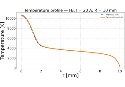
Elenbaas-Heller model for H₂ DC plasma — Cantera numerical solver.
Elenbaas-Heller model for H₂ DC plasma — Cantera numerical solver.
Use Stine-Watson model for a DC thermal plasma in H₂.
Use Stine-Watson model for a DC thermal plasma in H₂.- thermo_transport_data: rizer.io.thermo_transport_data_reader.ThermoTransportDataReader#
Thermo-transport data reader for the specified gas, pressure, and source.
- radiation_data: rizer.io.radiation_data_reader.RadiationDataReader#
Radiation data reader for the specified gas, pressure, source, and emission radius.
- idx_high_temp#
- property a_sigma: float#
Fitted parameter \(a_\sigma\) in (S/m)/(W.m^-1).
See
fit_electrical_conductivity()for details.
- property theta_sigma: float#
Fitted parameter \(\theta_\sigma\) in W.m^-1.
See
fit_electrical_conductivity()for details.
- property a_h: float#
Fitted parameter \(a_h\) in (J/kg)/(W.m^-1).
See
fit_enthalpy()for details.
- property a_eps: float#
Fitted parameter \(a_\varepsilon\) in (W.m^-3.sr^-1)/(W.m^-1).
See
fit_nec()for details.
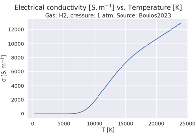
- fit_electrical_conductivity(sigma_cutoff: float = 100.0, plot_fit: bool = True) tuple[float, float]#
Fit the electrical conductivity.
The electrical conductivity is fitted to a linear function for the data above the cutoff.
- Parameters:
- Returns:
Fitted parameters:
\(a_\sigma\) in (S/m)/(W.m^-1)
\(\theta_\sigma\) in W.m^-1
- Return type:
Notes
The electrical conductivity \(\sigma\) is assumed to be linear above the cutoff:
\[\begin{split}\sigma(\theta)= \begin{cases} 0 & \text { for } \theta<\theta_\sigma \\ a_\sigma\left(\theta-\theta_\sigma\right) & \text { for } \theta>\theta_\sigma \end{cases}\end{split}\]where:
\(\theta\) is the thermal conductivity in W.m^-1.K^-1,
\(a_\sigma\) is the electrical conductivity coefficient in (S/m)/(W.m^-1),
\(\theta_\sigma\) is the electrical conductivity threshold in W.m^-1,
\(\sigma\) is the electrical conductivity in S/m.
- fit_enthalpy(plot_fit: bool = True) float#
Fit the enthalpy.
- Parameters:
plot_fit (
bool, optional) – If True, plot the fit, by default True.- Returns:
Fitted parameter \(a_h\) in (J/kg)/(W.m^-1).
- Return type:
Notes
The enthalpy \(h\) is assumed to be linear with respect to the integrated thermal conductivity:
\[h(\theta) = a_h \theta\]where:
\(\theta\) is the thermal conductivity in W.m^-1.K^-1,
\(a_h\) is the enthalpy coefficient in (J/kg)/(W.m^-1),
\(h\) is the enthalpy in J/kg.
- fit_nec(theta_sigma: float | None = None, plot_fit: bool = True) float#
Fit the Net Emission Coefficient (NEC).
- Parameters:
- Returns:
Fitted parameter \(a_\varepsilon\) in (W.m^-3.sr^-1)/(W.m^-1).
- Return type:
Notes
The NEC is assumed to be linear is assumed to be linear above the SAME cutoff as the electrical conductivity:
\[\begin{split}\varepsilon_N(\theta)= \begin{cases} 0 & \text { for } \theta<\theta_\sigma \\ a_{\varepsilon}\left(\theta-\theta_\sigma\right) & \text { for } \theta>\theta_\sigma \end{cases}\end{split}\]where:
\(\theta\) is the thermal conductivity in W.m^-1.K^-1,
\(a_\varepsilon\) is the NEC coefficient in (W.m^-3.sr^-1)/(W.m^-1),
\(\theta_\sigma\) is the electrical conductivity threshold in W.m^-1,
\(\varepsilon_N\) is the NEC in W.m^-3.sr^-1.