—

Elenbaas-Heller model for H₂ DC plasma.

This example demonstrates how to use the Elenbaas-Heller model to compute the temperature and integrated thermal conductivity in a DC plasma.

The Elenbaas-Heller model is a simple analytical model that describes the temperature distribution in a DC plasma torch, at low pressure (typically 1 atm), stabilized by water-cooled walls.

Once the temperature distribution is known, the conductivity of the channel can be determined.

It is based on the following assumptions:

• no mass flow in the plasma,

• the plasma is in a steady state and is axially symmetric,

• there is no magnetic field,

• the plasma is in thermal and chemical equilibrium,

• gravity, viscous dissipation and thermodiffusion effects are negligible,

• there is a cold zone (where the electrical conductivity is zero) around a hot zone (where the electrical conductivity is linear with the integrated thermal conductivity),

• Here, the radiative power is neglected (since we are only considering low pressure plasma),

• pressure is assumed to be constant (at atmospheric pressure).

In this example, we use the Elenbaas-Heller model, extended by Gueye to compute the temperature and integrated thermal conductivity in a H₂ DC plasma. We first load the transport data from a file and plot the electrical conductivity and thermal conductivity as a function of temperature. We then define the Elenbaas-Heller model and use it to compute the temperature and integrated thermal conductivity as a function of the radial distance. Finally, we plot the temperature as a function of the radial distance for different current values.

Notes

The Elenbaas-Heller models a DC plasma, by solving the following equation (see [Gueye2017] and [Elenbaas1951] for details):

\[\frac{1}{r} \frac{d}{dr} \left( r \kappa(T) \frac{dT}{dr} \right) + \sigma(T) E^2 + P^{rad}(T)= 0\]

where:

• \(r\) is the radial distance,

• \(\kappa(T)\) is the thermal conductivity,

• \(T\) is the temperature,

• \(\sigma(T)\) is the electrical conductivity,

• \(E\) is the electric field,

• \(P^{rad}(T)\) is the radiative power.

Introducing the integrated thermal conductivity \(\Theta(T) = \int_0^T \kappa(s) ds\), and neglecting the radiative power, we can rewrite the equation as:

\[\frac{1}{r} \frac{d}{dr} \left( r \frac{d\Theta}{dr} \right) + \sigma(\Theta) E^2 = 0\]

As [Gueye2017] noted, the electrical conductivity of hydrogen can be written as a linear function of the integrated thermal conductivity:

\[\begin{split}\sigma(\Theta) = \begin{cases} 0 & \text{if } \Theta < \theta_\sigma (r \in ]r_0, R])\\ a_\sigma (\Theta - \theta_\sigma) & \text{if } \Theta \geq \theta_\sigma (r \in [0, r_0]) \end{cases}\end{split}\]

where:

• \(a_\sigma\) is the slope of the electrical conductivity vs. integrated thermal conductivity, in (S/m)/(W.m^-1),

• \(\theta_\sigma\) is the first value of the integrated thermal conductivity where the electrical conductivity is non-zero, in W/m,

• \(r_0\) is the inner (arc) radius, in m, such that radius lower than \(r_0\) corresponds to non-zero electrical conductivity, and radius greater than \(r_0\) corresponds to zero electrical conductivity,

• \(R\) is the outer (torch) radius, in m.

We now see that there is a cold zone (where the electrical conductivity is zero) and a hot zone (where the electrical conductivity is linear with the integrated thermal conductivity).

With the following boundary conditions:

• Assuming the wall is maintened at 0 K, \(\Theta(r=R) = \int_0^{T(R)=T_w=0} \kappa(s) ds = 0\).

• By symmetry, \(\frac{d\Theta}{dr}(r=0) = \left( \frac{dT}{dr} \lambda(T) \right)(r=0) = 0\).

• By continuity, \(\Theta(r_0^-) = \Theta(r_0^+) = \theta_\sigma\).

• And by continuity of the derivative, \(\frac{d\Theta}{dr}(r_0^-) = \frac{d\Theta}{dr}(r_0^+)\).

The analytical solution to the Elenbaas-Heller equation is then given by:

\[\begin{split}\Theta(r) = \begin{cases} \theta_\sigma \left( 1 + \frac{J_0(\epsilon r)}{J_1(\epsilon r_0)} \frac{1}{r_0 \epsilon \ln(R/r_0)} \right) & \text{if } r \in [0, r_0]\\ \theta_\sigma \frac{\ln(r/R)}{\ln(r_0/R)} & \text{if } r \in ]r_0, R] \end{cases}\end{split}\]

where:

• \(\epsilon = \sqrt{a_\sigma E^2}\),

• \(J_0\) is the Bessel function of the first kind of order 0,

• \(J_1\) is the Bessel function of the first kind of order 1.

See Also

ElenbaasHeller

Tags: plasma Elenbaas-Heller DC plasma thermal conductivity electrical conductivity VAC

# This is an option for the online documentation, so that each image is displayed separately.
# sphinx_gallery_multi_image = "single"

Import the required libraries.

import matplotlib.pyplot as plt
import numpy as np
import seaborn as sns

from rizer.thermal_plasma.elenbaas_heller import ElenbaasHeller
from rizer.thermal_plasma.fit_LTE_data import FitLTEData

sns.set_theme("poster")

Load transport data and plot them.

# Load data.
H2_lte_data = FitLTEData(
    gas_name_transport="H2",
    gas_name_radiation="H2",
    pressure_atm=1,
    source_transport="Boulos2023",
    source_radiation="Gueye2017",
    emission_radius_mm=0,
    max_temperature_fit=12000.0,
)

# Plot electrical conductivity vs. temperature.
H2_lte_data.thermo_transport_data.plot(x="T", y="sigma")
# Plot thermal conductivity vs. temperature.
H2_lte_data.thermo_transport_data.plot(x="T", y="kappa")

• 
• 

/home/runner/work/rizer/rizer/rizer/thermal_plasma/fit_LTE_data.py:321: UserWarning: In `FitLTEData.fit_nec`, using previously fitted theta_sigma.
  warn("In `FitLTEData.fit_nec`, using previously fitted theta_sigma.")

(<Figure size 1200x800 with 1 Axes>, <Axes: title={'center': 'Gas: H2, pressure: 1 atm, Source: Boulos2023'}, xlabel='$\\mathregular{T}$ $\\mathregular{[K]}$', ylabel='$\\mathregular{\\kappa}$ $\\mathregular{[W.m^{-1}.K^{-1}]}$'>)

Define the Elenbaas-Heller model.

Note that the parameters electric_field and current are mutually exclusive. If you define one, the other must be set to None.

# Define the parameters.
R = 10e-3  # m
electric_field = 5000  # V/m
current = None  # A
# electric_field = None  # V/m
# current = 10  # A

# Define and resolve the Elenbaas-Heller model.
elenbaas = ElenbaasHeller(
    R,
    electric_field=electric_field,
    current=current,
    gas_data=H2_lte_data,
)

Plot the results in the approximation of the arc channel model.

\[\begin{split}\sigma(\Theta) = \begin{cases} 0 & \text{if } \Theta < \theta_\sigma (r \in ]r_0, R])\\ a (\Theta - \theta_\sigma) & \text{if } \Theta \geq \theta_\sigma (r \in [0, r_0]) \end{cases}\end{split}\]

# Define the radial distance.
r_values = np.linspace(0, R, num=1000, dtype=float)

# Print the parameters.
print(f"Outer radius R: {elenbaas._R:.2e} m")
print(f"a_sigma: {elenbaas.a_sigma:.2e} (S/m)/(W/m)")
print(f"theta_sigma: {elenbaas.theta_sigma:.2e} W/m")

# Compute the electrical conductivity.
theta = elenbaas.theta

# Plot the electrical conductivity vs. integrated thermal conductivity.
H2_lte_data.fit_electrical_conductivity(sigma_cutoff=100, plot_fit=True)

Outer radius R: 1.00e-02 m
a_sigma: 2.27e-01 (S/m)/(W/m)
theta_sigma: 2.99e+04 W/m

(np.float64(0.22699241092881833), 29894.450000000008)

Print electric field and current.

# Print the electric field.
print(f"Electric field: {elenbaas.electric_field:.2e} V/m")
# Compute and print the current.
current = elenbaas.analytical_current()
print(f"Current: {current:.2e} A")

Electric field: 5.00e+03 V/m
Current: 1.64e+01 A

Compute and plot the theta values.

theta_values = np.array([elenbaas.analytical_theta_vs_radius(r) for r in r_values])

fig, ax = plt.subplots(figsize=(12, 8), layout="constrained")
ax.plot(r_values * 1e3, theta_values)
ax.set_xlabel("r [mm]")
ax.set_ylabel("Theta [W/m]")
ax.set_title("Integrated thermal conductivity [W/m] versus radial distance [mm]")
plt.show()

Compute and plot the temperature values.

temperature_values = np.array([elenbaas.get_temperature_vs_radius(r) for r in r_values])

fig, ax = plt.subplots(figsize=(12, 8), layout="constrained")
ax.plot(r_values * 1e3, temperature_values)
ax.set_xlabel("r [mm]")
ax.set_ylabel("Temperature [K]")
ax.set_title("Temperature [K] versus radial distance [mm]")
plt.show()

/home/runner/work/rizer/rizer/rizer/thermal_plasma/elenbaas_heller.py:340: RuntimeWarning: The iteration is not making good progress, as measured by the
 improvement from the last ten iterations.
  temperature = fsolve(f, initial_temperature)[0]

Plot temperature vs. radial distance.

Plot the temperature vs. radial distance for different current values.

# Define the current values.
intensity_values = [1, 5, 10, 20, 50, 100]  # A

# Define the figure.
fig, ax = plt.subplots(figsize=(12, 8), layout="constrained")

# Loop over the current values.
for current in intensity_values:
    # Define the Elenbaas-Heller model.
    elenbaas = ElenbaasHeller(
        R,
        electric_field=None,
        current=current,
        gas_data=H2_lte_data,
    )

    # Compute and plot the temperature values.
    temperature_values = np.array(
        [elenbaas.get_temperature_vs_radius(r) for r in r_values]
    )

    ax.plot(r_values * 1e3, temperature_values, label=f"Current: {current} A")

# Set the labels and title.
ax.set_xlabel("r [mm]")
ax.set_ylabel("Temperature [K]")
ax.set_title("Temperature [K] versus radial distance [mm] (R = 10 mm)")
ax.legend()
plt.show()

Plot electric fied vs. current.

The current is given by:

\[I=\iint_S \vec{j} \cdot d \vec{S}=\int_0^R 2 \pi r j(r) d r=2 \pi E \int_0^R \sigma(r) r d r\]

Then, using the computation of the temperature and electric conductivity, this expression reduces to:

\[I = \frac{2 \pi \theta_\sigma}{E \ln \left(R / r_0\right)}\]

where:

• \(I\) is the current,

• \(\theta_\sigma\) is the constant, initial value of the integrated thermal conductivity,

• \(E\) is the electric field,

• \(R\) is the outer radius (torch radius),

• \(r_0\) is the inner radius (arc radius), such that \(r_0 \sqrt{a E^2}\) is a zero of the Bessel function \(J_0\).

Plot the electric field vs. current for different outer radius.

# Define the outer radius values.
R_values = [10e-3, 20e-3, 50e-3]  # m.

# Define the current values.
current_values = np.linspace(5, 100, 100, dtype=float)  # A

# Define the figure.
fig, ax = plt.subplots(figsize=(12, 8), layout="constrained")


# Loop over the outer radius values.
for R in R_values:
    electric_field_values = np.zeros_like(current_values)

    for i, current in enumerate(current_values):
        # Define the Elenbaas-Heller model.
        elenbaas = ElenbaasHeller(
            R,
            electric_field=None,
            current=current,
            gas_data=H2_lte_data,
        )

        # Compute the electric field values.
        electric_field_values[i] = elenbaas.electric_field

    ax.plot(current_values, electric_field_values, label=f"R: {R * 1e3} mm")

# Set the labels and title.
ax.set_xlabel("Current [A]")
ax.set_ylabel("Electric field [V/m]")
ax.set_title("Electric field [V/m] versus current [A]")
ax.legend()
plt.show()

Also plot the tests.

from tests.thermal_plasma.test_elenbaas_heller import test_fig13a, test_fig13b  # noqa: E402, I001

Plot electric field vs. current.

test_fig13a(plot=True)

• 
• 
• 

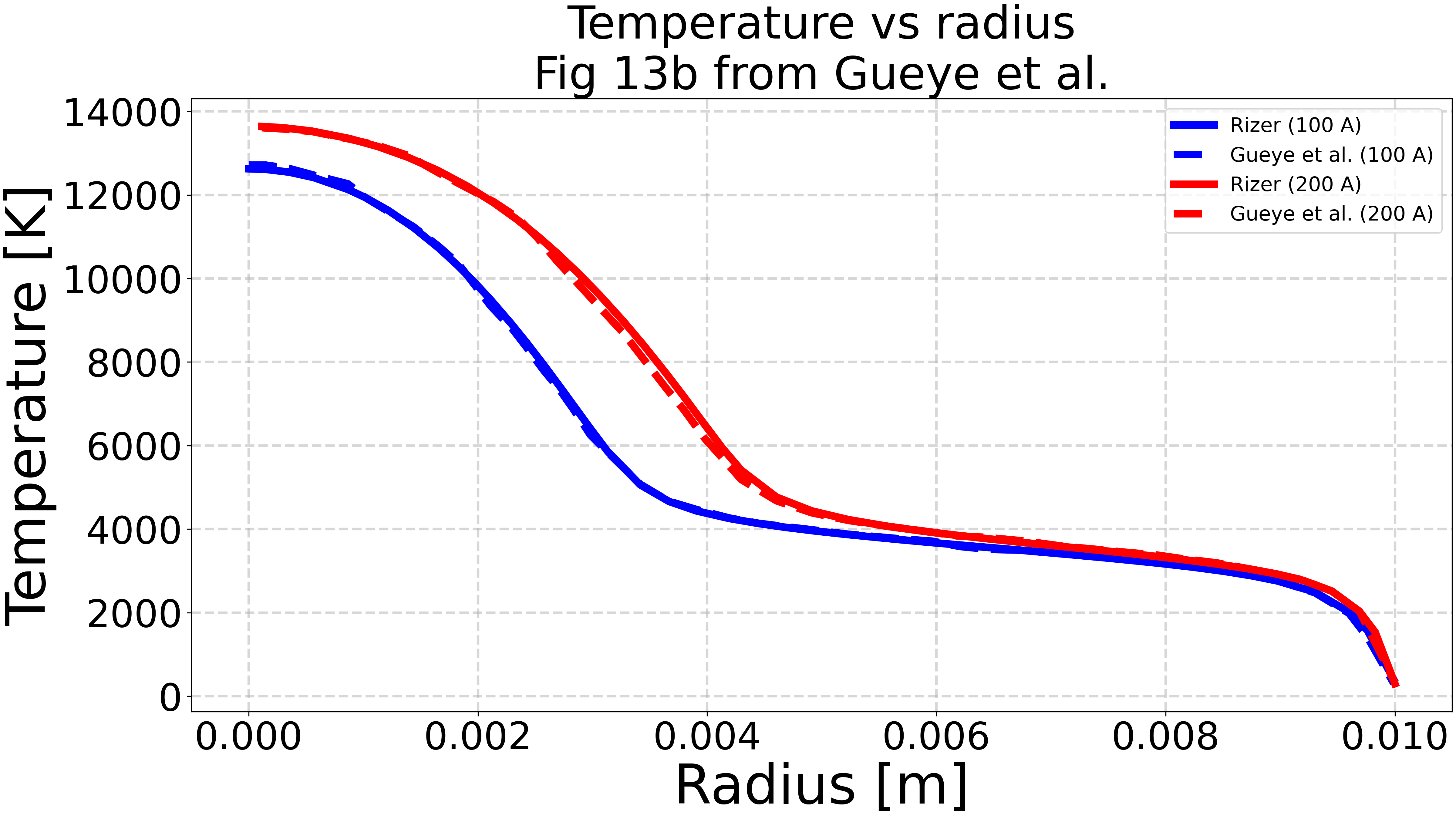
Plot temperature vs. radial distance for different current values.

test_fig13b(plot=True)

• 
• 
•