—

Plot thermodynamic properties of H₂ vs. temperatures.

This example shows how to compute and plot the mass enthalpy of a plasma of hydrogen (H₂) as a function of temperature. It also shows how to compute and plot the mole fractions of the main species in the plasma as a function of temperature, as well as the density and heat capacity.

The data for the mass enthalpy, density and heat capacity are compared to reference data from the literature.

Equilibrium composition

The following species are considered in the mechanism:

• H, H2

• corresponding ions,

• electrons,

Data comes from the following sources:

• [GRCDatabase] for H, H2, H+ and H2+, and for electrons,

The thermo data are given as NASA 9 polynomial coefficients (For details, see https://cantera.org/stable/reference/thermo/species-thermo.html#the-nasa-9-coefficient-polynomial-parameterization).

The temperature range is from 200 to 20000 K for atomic species, and from 200 to 6000 K for molecular species.

Then, to compute the equilibrium composition of the plasma, the Gibbs free energy minimization method is used.

References data

The reference data for the mass enthalpy and density of hydrogen at 1 atm are taken from:

• [Boulos2023] for the mass enthalpy, density and heat capacity.

• [MinPlasCalc] (& [minplascalcPaper]) for the mass enthalpy, density and heat capacity.

• [GRCDatabase] and [Burcat] for the mass enthalpy, density, heat capacity and equilibrium composition.

Tags: thermo hydrogen H2 plasma mass enthalpy density heat capacity ions electrons

Import the required libraries.

import cantera as ct
import matplotlib.pyplot as plt
import numpy as np

from rizer.io.thermo_transport_data_reader import ThermoTransportDataReader
from rizer.misc.plt_utils import get_species_in_latex, set_mpl_style
from rizer.misc.utils import get_path_to_data

# Set the style of the plots.
set_mpl_style(nb_columns=1)

Define the thermo data files to load.

mechanism = get_path_to_data("mechanisms", "Goutier2025", "CH4_to_C2H2.yaml")

# Load the gas phase.
gas = ct.Solution(
    mechanism,
    name="gas",
    transport_model=None,
)

Compute the equilibrium composition of the plasma at 1 atm and for a range of temperatures.

temperatures = np.linspace(300, 25000, 1000)
states = ct.SolutionArray(gas, shape=temperatures.shape)
states.TPX = temperatures, ct.one_atm, "H2:1"
states.equilibrate("TP")

Load reference data.

data_H2_Boulos2023 = ThermoTransportDataReader(
    gas_name="H2", pressure_atm=1, source="Boulos2023"
)
data_H2_minplascalc = ThermoTransportDataReader(
    gas_name="H2", pressure_atm=1, source="minplascalc"
)

Plot the mass enthalpy vs. temperature.

fig, ax = plt.subplots()
data_H2_Boulos2023.plot(
    x="T",
    y="h",
    fig_ax=(fig, ax),
    show=False,
    label="Boulos2023",
    ls="-",
    lw=4,
    color="black",
)
data_H2_minplascalc.plot(
    x="T",
    y="h",
    fig_ax=(fig, ax),
    show=False,
    label="MinPlasCalc",
    ls="--",
    color="red",
)
ax.plot(
    temperatures,
    states.enthalpy_mass,
    label="GRC+Burcat",
    ls=":",
    color="blue",
)
ax.legend(loc="lower right")
ax.set_yscale("log")
ax.set_ylim(1e7, 4e9)
ax.set_title(r"$\mathrm{H_2}$ in LTE at 1 atm", fontsize=30)

plt.show()

Plot the density vs. temperature.

fig, ax = plt.subplots()
data_H2_Boulos2023.plot(
    x="T",
    y="rho",
    fig_ax=(fig, ax),
    show=False,
    label="Boulos2023",
    ls="-",
    lw=4,
    color="black",
)
data_H2_minplascalc.plot(
    x="T",
    y="rho",
    fig_ax=(fig, ax),
    show=False,
    label="MinPlasCalc",
    ls="--",
    color="red",
)
ax.plot(
    temperatures,
    states.density_mass,
    label="GRC+Burcat",
    ls=":",
    color="blue",
)
ax.legend()
ax.set_yscale("log")
ax.set_title(r"$\mathrm{H_2}$ in LTE at 1 atm", fontsize=30)

plt.show()

Plot the heat capacity vs. temperature.

We see some differences between the reference data and the computed data. The difference is probably due to “total” heat capacity in the reference data, while the computed data is the “non-reactive” heat capacity.

fig, ax = plt.subplots()
data_H2_Boulos2023.plot(
    x="T",
    y="cp",
    fig_ax=(fig, ax),
    show=False,
    label="Boulos2023",
    ls="-",
    lw=4,
    color="black",
)
data_H2_minplascalc.plot(
    x="T",
    y="cp",
    fig_ax=(fig, ax),
    show=False,
    label="MinPlasCalc",
    ls="--",
    color="red",
)
ax.plot(
    temperatures,
    states.cp_mass,
    label="GRC+Burcat ($c_{p, \text{eq}}$)",
    ls=":",
    color="blue",
)
ax.plot(
    temperatures,
    np.gradient(states.enthalpy_mass, temperatures),
    label=r"GRC+Burcat ($c_{p, \text{eq}} =\frac{d h}{d T}$)",
    ls=":",
    color="cyan",
)
ax.legend(loc="lower right", fontsize=20)
ax.set_yscale("log")
ax.set_title(r"$\mathrm{H_2}$ in LTE at 1 atm", fontsize=30)

plt.show()

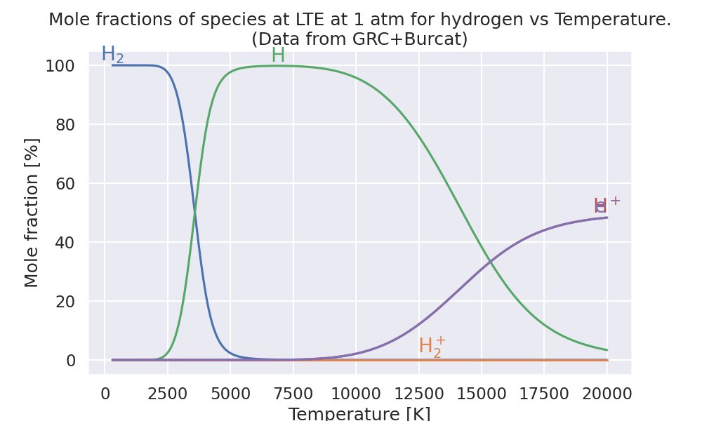
Plot mole fractions vs. temperature.

main_species = ["H2", "H2+", "H", "H+", "e-"]
fig, ax = plt.subplots()

for species in main_species:
    ax.plot(temperatures, states(species).X * 100, label=species)

    # Annotate the maximum mole fraction, with the same color as the line.
    x_max = temperatures[np.argmax(states(species).X)]
    y_max = np.max(states(species).X) * 100
    color = plt.gca().lines[-1].get_color()
    ax.text(
        x_max,
        y_max,
        s=get_species_in_latex(species),
        horizontalalignment="center",
        verticalalignment="bottom",
        color=color,
    )

ax.set_xlabel("Temperature [K]")
ax.set_ylabel("Mole fraction [%]")
ax.set_title(
    "Mole fractions of species at LTE at 1 atm for hydrogen vs Temperature.\n"
    "(Data from GRC+Burcat)"
)
plt.show()