—
Plot electrical conductivity vs. temperature for a plasma of methane.#
The electrical conductivity of a plasma is the ability of the plasma to conduct an electric current. It is a key parameter in the study of plasmas, as it determines the behavior of the plasma in the presence of an electric field.
It assumed that the plasma is in local thermodynamic equilibrium (LTE), which means that all temperatures are equal.
Equilibrium composition#
The following species are considered in the mechanism:
H, H2, C, CH, CH2, CH3, CH4, C2, C2H, C2H2, C2H3, C2H4, C2H5, C2H6,
corresponding ions,
electrons,
no solid carbon species.
Data comes from the following sources:
[GRCDatabase] for neutral species, C+, C2+, CH+, H+ and H2+, and for electrons,
[Burcat] for the other ions.
The thermo data are given as NASA 9 polynomial coefficients (For details, see https://cantera.org/stable/reference/thermo/species-thermo.html#the-nasa-9-coefficient-polynomial-parameterization).
The temperature range is from 200 to 20000 K for atomic species, and from 200 to 6000 K for molecular species.
Then, to compute the equilibrium composition of the plasma, the Gibbs free energy minimization method is used.
Electrical conductivity computation#
The computation presented here is based on [Raizer1991] and on Chapter II, section 13 of [Mitchner1973].
The electrical conductivity is given by:
where:
\(n_e\) is the electron number density,
\(e\) is the elementary charge,
\(m_e\) is the electron mass,
\(\large \overline{\nu_{eH}} = \sum_k \overline{\nu_{ek}}\) is the average momentum transfer collision frequency of an electron with all heavy particles.
\(\large \overline{\nu_{ek}}\) is the energy-weighted average momentum transfer collision frequency between an electron and heavy particles of species k,
\(\large \overline{\nu_{eH}}\) can be computed as a sum of the collision frequencies with neutrals \(\large \overline{\nu_{eN}}\) and with ions \(\large \overline{\nu_{eI}}\):
\(\large \overline{\nu_{eH}} = \overline{\nu_{eN}} + \overline{\nu_{eI}}\).
In the special case where \(\large \overline{\nu_{eI}} >> \overline{\nu_{eN}}\), the plasma is said to be strongly ionized, and the electrical conductivity can be computed using the Spitzer formula:
where:
\(\sigma_{\text{strongly ionized}}\) is the strongly ionized electrical conductivity,
\(\text{Spitzer constant} = 1.53 \times 10^{-2} \, \Omega^{-1} \, \text{m}^{-1} \, \text{K}^{-3/2}\),
\(T_e\) is the electron temperature,
\(\log(\Lambda)\) is the Coulomb logarithm.
The Spitzer constant depends on the effective charge of the ions in the plasma and can be computed using the formula given in [WikiSpitzerResistivity].
The energy-weighted average momentum transfer collision frequency between an electron and heavy particle k is:
where:
\(n_k\) is the number density of heavy particles of species k,
\(v_{th, e}\) is the electron thermal velocity,
\(\large \overline{Q_{ek}}\) is the average momentum-transfer cross section (as defined in Section 6 of chapter II of [Mitchner1973]).
Comparisons are made for the various models of cross-sections:
Hard sphere model: cross sections are computed assuming that species are hard spheres, with a specified effective radius.
Tabulated model CH4: The only species considered is methane, and the cross section is computed using tabulated data of cross sections vs. energy
Tabulated model all: When available, a tabulated cross section is used for species. If no tabulated data is available, a hard sphere model is used with a default effective radius of 1e-10 m. Ions cross sections are computed using the Rutherford model, with the Coulomb potential. The total collision frequency is computed as a sum of the collision frequencies with all species, including ions.
The differents electrical conductivities resulting from these models are compared to the data of [Niu2016].
Import the required libraries.#
import cantera as ct
import matplotlib.pyplot as plt
import numpy as np

import rizer.misc.units as u
from rizer.io.thermo_transport_data_reader import ThermoTransportDataReader
from rizer.misc.ct_utils import load_goutier2025_mechanism
from rizer.misc.plt_utils import get_text, set_mpl_style
from rizer.plasma.collision_frequency import (
    IonMomentumTransferCollisionFrequencyModel,
    MomentumTransferCollisionFrequencyModel,
    get_momentum_transfer_collision_frequency_model,
)
from rizer.plasma.momentum_transfer_cross_sections import (
    HardSphereCrossSection,
    MomentumTransferCrossSectionModel,
    get_momentum_transfer_cross_section_model,
)

set_mpl_style(nb_columns=1)
Define the thermo data files to load.#
gas = load_goutier2025_mechanism("gas")
Define the temperature range and the pressure.#
temperatures = np.linspace(300, 30000, 1000, dtype=float)  # K
pressure = ct.one_atm  # Pa
Create the models for the elastic cross sections.#
# Hard sphere model.
effective_radius = 1e-10  # m
model_1 = HardSphereCrossSection(effective_radius)
effective_radius = 3.5e-10  # m
model_2 = HardSphereCrossSection(effective_radius)

# Tabulated model, based on CH4 data.
model_3 = get_momentum_transfer_cross_section_model(
    species="CH4",
    database_to_use="Morgan.txt",
)

# Tabulated model, based on all available data.
species_list = gas.species_names
ions_list = [species for species in species_list if gas.species(species).charge > 0]
model_4 = [
    get_momentum_transfer_collision_frequency_model(
        species=species,
        use_default_radius=True,
        use_first_available=True,
        default_radius=1e-10,
    )
    for species in species_list
]

models: list[MomentumTransferCrossSectionModel] = [
    model_1,
    model_2,
    model_3,
]
Compute the electrical conductivity.#
electrical_conductivities = np.zeros((len(temperatures), len(models) + 1))

for i, T in enumerate(temperatures):
    # Set temperature, pressure and composition of the gas.
    gas.TPX = T, pressure, "CH4:1"

    # Equilibrate the gas.
    gas.equilibrate("TP")

    # Get the mole fraction dictionary.
    mfd = gas.mole_fraction_dict()

    # Get the total number density, assuming ideal gas behavior and LTE.
    n_tot = pressure / (u.k_b * T)  # m^-3

    # Get the mole fractions of the electrons.
    x_e = mfd["e-"]
    # Compute the number density of electrons.
    n_e = x_e * n_tot  # m^-3

    # For the 3 first models, CH4 is the only species considered.
    # The other species are electrons and CH4+.
    n_CH4 = (1 - 2 * x_e) * n_tot  # m^-3

    for j, model in enumerate(models):
        # Get the momentum transfer collision frequency between electrons and neutrals.
        nu_neutral_model = MomentumTransferCollisionFrequencyModel(
            name=model.name,
            cross_section_model=model,
        )
        nu_en = nu_neutral_model.get_mean_momentum_transfer_collision_frequency(
            T, n_CH4, n_e=n_e
        )

        # Get the momentum transfer collision frequency between electrons and ions.
        nu_ion_model = IonMomentumTransferCollisionFrequencyModel(name=model.name, Z=1)
        nu_ei = nu_ion_model.get_mean_momentum_transfer_collision_frequency(
            T, n_h=n_e, n_e=n_e
        )

        # Compute the total collision frequency.
        nu = nu_en + nu_ei

        # Compute the total electrical conductivity.
        σ_total = u.e**2 * n_e / (u.m_e * nu)  # S/m

        electrical_conductivities[i, j] = σ_total

    # For the last model, use a more complete model.
    # Compute the total collision frequency.
    nu_tot = 0.0
    # Compute the total collision frequency for ions.
    nu_tot_ions = 0.0
    for k, species in enumerate(species_list):
        if species == "e-":
            # Skip electrons.
            continue

        if species not in mfd:
            print(
                f"Species {species} not found in mole fraction dictionary, at T={T} K."
            )
            continue

        x_k = mfd[species]
        n_k = x_k * n_tot  # m^-3

        nu = model_4[k].get_mean_momentum_transfer_collision_frequency(
            T, n_h=n_k, n_e=n_e
        )
        nu_tot += nu
        if species in ions_list:
            nu_tot_ions += nu

    # Compute the total electrical conductivity.
    σ_total = u.e**2 * n_e / (u.m_e * nu_tot)  # S/m

    # If the number density of ions is greater than the number density of neutrals,
    # we can assume that the plasma is strongly ionized.
    nu_tot_neutrals = nu_tot - nu_tot_ions
    if nu_tot_ions > 2 * nu_tot_neutrals:
        X_k = np.array(
            [
                gas.X[i] if species in ions_list else 0
                for i, species in enumerate(species_list)
            ]
        )
        Z_k = np.array(
            [
                gas.species(species).charge if species in ions_list else 0
                for species in species_list
            ]
        )
        Z_eff = np.sum(X_k * Z_k**2) / np.sum(X_k * Z_k)
        # See [WikiSpitzerResistivity]_
        F = (1 + 1.198 * Z_eff + 0.222 * Z_eff**2) / (
            1 + 2.966 * Z_eff + 0.753 * Z_eff**2
        )
        print(
            f"At T={T} K, the plasma is strongly ionized, "
            f"with Z_eff={Z_eff:.2f}, giving F={F:.2f} (1/F={1 / F:.2f})."
        )
        σ_total /= F  # Spitzer constant for strongly ionized plasma, see (II 13.18) of [Mitchner1973]_.

    electrical_conductivities[i, len(models)] = σ_total
Species C2H+ not found in mole fraction dictionary, at T=300.0 K.
Species CH+ not found in mole fraction dictionary, at T=300.0 K.
Species C2+ not found in mole fraction dictionary, at T=300.0 K.
Species C+ not found in mole fraction dictionary, at T=300.0 K.
Species C++ not found in mole fraction dictionary, at T=300.0 K.
Species C+++ not found in mole fraction dictionary, at T=300.0 K.
Species C2+ not found in mole fraction dictionary, at T=329.72972972972974 K.
Species C++ not found in mole fraction dictionary, at T=329.72972972972974 K.
Species C+++ not found in mole fraction dictionary, at T=329.72972972972974 K.
Species C++ not found in mole fraction dictionary, at T=359.4594594594595 K.
Species C+++ not found in mole fraction dictionary, at T=359.4594594594595 K.
Species C++ not found in mole fraction dictionary, at T=389.18918918918916 K.
Species C+++ not found in mole fraction dictionary, at T=389.18918918918916 K.
Species C++ not found in mole fraction dictionary, at T=418.9189189189189 K.
Species C+++ not found in mole fraction dictionary, at T=418.9189189189189 K.
Species C++ not found in mole fraction dictionary, at T=448.64864864864865 K.
Species C+++ not found in mole fraction dictionary, at T=448.64864864864865 K.
Species C++ not found in mole fraction dictionary, at T=478.3783783783784 K.
Species C+++ not found in mole fraction dictionary, at T=478.3783783783784 K.
Species C++ not found in mole fraction dictionary, at T=508.1081081081081 K.
Species C+++ not found in mole fraction dictionary, at T=508.1081081081081 K.
Species C++ not found in mole fraction dictionary, at T=537.8378378378378 K.
Species C+++ not found in mole fraction dictionary, at T=537.8378378378378 K.
Species C++ not found in mole fraction dictionary, at T=567.5675675675675 K.
Species C+++ not found in mole fraction dictionary, at T=567.5675675675675 K.
Species C++ not found in mole fraction dictionary, at T=597.2972972972973 K.
Species C+++ not found in mole fraction dictionary, at T=597.2972972972973 K.
Species C++ not found in mole fraction dictionary, at T=627.0270270270271 K.
Species C+++ not found in mole fraction dictionary, at T=627.0270270270271 K.
Species C++ not found in mole fraction dictionary, at T=656.7567567567568 K.
Species C+++ not found in mole fraction dictionary, at T=656.7567567567568 K.
Species C++ not found in mole fraction dictionary, at T=686.4864864864865 K.
Species C+++ not found in mole fraction dictionary, at T=686.4864864864865 K.
Species C++ not found in mole fraction dictionary, at T=716.2162162162163 K.
Species C+++ not found in mole fraction dictionary, at T=716.2162162162163 K.
Species C+++ not found in mole fraction dictionary, at T=745.9459459459459 K.
Species C+++ not found in mole fraction dictionary, at T=775.6756756756756 K.
Species C+++ not found in mole fraction dictionary, at T=805.4054054054054 K.
Species C+++ not found in mole fraction dictionary, at T=835.1351351351351 K.
Species C+++ not found in mole fraction dictionary, at T=864.8648648648649 K.
Species C+++ not found in mole fraction dictionary, at T=894.5945945945946 K.
Species C+++ not found in mole fraction dictionary, at T=924.3243243243244 K.
Species C+++ not found in mole fraction dictionary, at T=954.0540540540541 K.
Species C+++ not found in mole fraction dictionary, at T=983.7837837837837 K.
Species C+++ not found in mole fraction dictionary, at T=1013.5135135135135 K.
Species C+++ not found in mole fraction dictionary, at T=1043.2432432432433 K.
Species C+++ not found in mole fraction dictionary, at T=1072.972972972973 K.
Species C+++ not found in mole fraction dictionary, at T=1102.7027027027027 K.
Species C+++ not found in mole fraction dictionary, at T=1132.4324324324325 K.
Species C+++ not found in mole fraction dictionary, at T=1162.162162162162 K.
Species C+++ not found in mole fraction dictionary, at T=1191.8918918918919 K.
Species C+++ not found in mole fraction dictionary, at T=1221.6216216216217 K.
Species C+++ not found in mole fraction dictionary, at T=1251.3513513513512 K.
Species C+++ not found in mole fraction dictionary, at T=1281.081081081081 K.
Species C+++ not found in mole fraction dictionary, at T=1310.8108108108108 K.
Species C+++ not found in mole fraction dictionary, at T=1340.5405405405406 K.
Species C+++ not found in mole fraction dictionary, at T=1370.2702702702702 K.
Species C+++ not found in mole fraction dictionary, at T=1400.0 K.
Species C+++ not found in mole fraction dictionary, at T=1429.7297297297298 K.
At T=8624.324324324325 K, the plasma is strongly ionized, with Z_eff=1.00, giving F=0.51 (1/F=1.95).
At T=8654.054054054053 K, the plasma is strongly ionized, with Z_eff=1.00, giving F=0.51 (1/F=1.95).
At T=8683.783783783783 K, the plasma is strongly ionized, with Z_eff=1.00, giving F=0.51 (1/F=1.95).
At T=8713.513513513513 K, the plasma is strongly ionized, with Z_eff=1.00, giving F=0.51 (1/F=1.95).
At T=8743.243243243243 K, the plasma is strongly ionized, with Z_eff=1.00, giving F=0.51 (1/F=1.95).
At T=8772.972972972973 K, the plasma is strongly ionized, with Z_eff=1.00, giving F=0.51 (1/F=1.95).
At T=8802.702702702703 K, the plasma is strongly ionized, with Z_eff=1.00, giving F=0.51 (1/F=1.95).
At T=8832.432432432432 K, the plasma is strongly ionized, with Z_eff=1.00, giving F=0.51 (1/F=1.95).
At T=8862.162162162162 K, the plasma is strongly ionized, with Z_eff=1.00, giving F=0.51 (1/F=1.95).
At T=8891.891891891892 K, the plasma is strongly ionized, with Z_eff=1.00, giving F=0.51 (1/F=1.95).
At T=8921.621621621622 K, the plasma is strongly ionized, with Z_eff=1.00, giving F=0.51 (1/F=1.95).
At T=8951.351351351352 K, the plasma is strongly ionized, with Z_eff=1.00, giving F=0.51 (1/F=1.95).
At T=8981.081081081082 K, the plasma is strongly ionized, with Z_eff=1.00, giving F=0.51 (1/F=1.95).
At T=9010.810810810812 K, the plasma is strongly ionized, with Z_eff=1.00, giving F=0.51 (1/F=1.95).
At T=9040.54054054054 K, the plasma is strongly ionized, with Z_eff=1.00, giving F=0.51 (1/F=1.95).
At T=9070.27027027027 K, the plasma is strongly ionized, with Z_eff=1.00, giving F=0.51 (1/F=1.95).
At T=9100.0 K, the plasma is strongly ionized, with Z_eff=1.00, giving F=0.51 (1/F=1.95).
At T=9129.72972972973 K, the plasma is strongly ionized, with Z_eff=1.00, giving F=0.51 (1/F=1.95).
At T=9159.45945945946 K, the plasma is strongly ionized, with Z_eff=1.00, giving F=0.51 (1/F=1.95).
At T=9189.18918918919 K, the plasma is strongly ionized, with Z_eff=1.00, giving F=0.51 (1/F=1.95).
At T=9218.918918918918 K, the plasma is strongly ionized, with Z_eff=1.00, giving F=0.51 (1/F=1.95).
At T=9248.648648648648 K, the plasma is strongly ionized, with Z_eff=1.00, giving F=0.51 (1/F=1.95).
At T=9278.378378378378 K, the plasma is strongly ionized, with Z_eff=1.00, giving F=0.51 (1/F=1.95).
At T=9308.108108108108 K, the plasma is strongly ionized, with Z_eff=1.00, giving F=0.51 (1/F=1.95).
At T=9337.837837837838 K, the plasma is strongly ionized, with Z_eff=1.00, giving F=0.51 (1/F=1.95).
At T=9367.567567567568 K, the plasma is strongly ionized, with Z_eff=1.00, giving F=0.51 (1/F=1.95).
At T=9397.297297297297 K, the plasma is strongly ionized, with Z_eff=1.00, giving F=0.51 (1/F=1.95).
At T=9427.027027027027 K, the plasma is strongly ionized, with Z_eff=1.00, giving F=0.51 (1/F=1.95).
At T=9456.756756756757 K, the plasma is strongly ionized, with Z_eff=1.00, giving F=0.51 (1/F=1.95).
At T=9486.486486486487 K, the plasma is strongly ionized, with Z_eff=1.00, giving F=0.51 (1/F=1.95).
At T=9516.216216216217 K, the plasma is strongly ionized, with Z_eff=1.00, giving F=0.51 (1/F=1.95).
At T=9545.945945945947 K, the plasma is strongly ionized, with Z_eff=1.00, giving F=0.51 (1/F=1.95).
At T=9575.675675675675 K, the plasma is strongly ionized, with Z_eff=1.00, giving F=0.51 (1/F=1.95).
At T=9605.405405405405 K, the plasma is strongly ionized, with Z_eff=1.00, giving F=0.51 (1/F=1.95).
At T=9635.135135135135 K, the plasma is strongly ionized, with Z_eff=1.00, giving F=0.51 (1/F=1.95).
At T=9664.864864864865 K, the plasma is strongly ionized, with Z_eff=1.00, giving F=0.51 (1/F=1.95).
At T=9694.594594594595 K, the plasma is strongly ionized, with Z_eff=1.00, giving F=0.51 (1/F=1.95).
At T=9724.324324324325 K, the plasma is strongly ionized, with Z_eff=1.00, giving F=0.51 (1/F=1.95).
At T=9754.054054054053 K, the plasma is strongly ionized, with Z_eff=1.00, giving F=0.51 (1/F=1.95).
At T=9783.783783783783 K, the plasma is strongly ionized, with Z_eff=1.00, giving F=0.51 (1/F=1.95).
At T=9813.513513513513 K, the plasma is strongly ionized, with Z_eff=1.00, giving F=0.51 (1/F=1.95).
At T=9843.243243243243 K, the plasma is strongly ionized, with Z_eff=1.00, giving F=0.51 (1/F=1.95).
At T=9872.972972972973 K, the plasma is strongly ionized, with Z_eff=1.00, giving F=0.51 (1/F=1.95).
At T=9902.702702702703 K, the plasma is strongly ionized, with Z_eff=1.00, giving F=0.51 (1/F=1.95).
At T=9932.432432432432 K, the plasma is strongly ionized, with Z_eff=1.00, giving F=0.51 (1/F=1.95).
At T=9962.162162162162 K, the plasma is strongly ionized, with Z_eff=1.00, giving F=0.51 (1/F=1.95).
At T=9991.891891891892 K, the plasma is strongly ionized, with Z_eff=1.00, giving F=0.51 (1/F=1.95).
At T=10021.621621621622 K, the plasma is strongly ionized, with Z_eff=1.00, giving F=0.51 (1/F=1.95).
At T=10051.351351351352 K, the plasma is strongly ionized, with Z_eff=1.00, giving F=0.51 (1/F=1.95).
At T=10081.081081081082 K, the plasma is strongly ionized, with Z_eff=1.00, giving F=0.51 (1/F=1.95).
At T=10110.810810810812 K, the plasma is strongly ionized, with Z_eff=1.00, giving F=0.51 (1/F=1.95).
At T=10140.54054054054 K, the plasma is strongly ionized, with Z_eff=1.00, giving F=0.51 (1/F=1.95).
At T=10170.27027027027 K, the plasma is strongly ionized, with Z_eff=1.00, giving F=0.51 (1/F=1.95).
At T=10200.0 K, the plasma is strongly ionized, with Z_eff=1.00, giving F=0.51 (1/F=1.95).
At T=10229.72972972973 K, the plasma is strongly ionized, with Z_eff=1.00, giving F=0.51 (1/F=1.95).
At T=10259.45945945946 K, the plasma is strongly ionized, with Z_eff=1.00, giving F=0.51 (1/F=1.95).
At T=10289.18918918919 K, the plasma is strongly ionized, with Z_eff=1.00, giving F=0.51 (1/F=1.95).
At T=10318.918918918918 K, the plasma is strongly ionized, with Z_eff=1.00, giving F=0.51 (1/F=1.95).
At T=10348.648648648648 K, the plasma is strongly ionized, with Z_eff=1.00, giving F=0.51 (1/F=1.95).
At T=10378.378378378378 K, the plasma is strongly ionized, with Z_eff=1.00, giving F=0.51 (1/F=1.95).
At T=10408.108108108108 K, the plasma is strongly ionized, with Z_eff=1.00, giving F=0.51 (1/F=1.95).
At T=10437.837837837838 K, the plasma is strongly ionized, with Z_eff=1.00, giving F=0.51 (1/F=1.95).
At T=10467.567567567568 K, the plasma is strongly ionized, with Z_eff=1.00, giving F=0.51 (1/F=1.95).
At T=10497.297297297297 K, the plasma is strongly ionized, with Z_eff=1.00, giving F=0.51 (1/F=1.95).
At T=10527.027027027027 K, the plasma is strongly ionized, with Z_eff=1.00, giving F=0.51 (1/F=1.95).
At T=10556.756756756757 K, the plasma is strongly ionized, with Z_eff=1.00, giving F=0.51 (1/F=1.95).
At T=10586.486486486487 K, the plasma is strongly ionized, with Z_eff=1.00, giving F=0.51 (1/F=1.95).
At T=10616.216216216217 K, the plasma is strongly ionized, with Z_eff=1.00, giving F=0.51 (1/F=1.95).
At T=10645.945945945947 K, the plasma is strongly ionized, with Z_eff=1.00, giving F=0.51 (1/F=1.95).
At T=10675.675675675675 K, the plasma is strongly ionized, with Z_eff=1.00, giving F=0.51 (1/F=1.95).
At T=10705.405405405405 K, the plasma is strongly ionized, with Z_eff=1.00, giving F=0.51 (1/F=1.95).
At T=10735.135135135135 K, the plasma is strongly ionized, with Z_eff=1.00, giving F=0.51 (1/F=1.95).
At T=10764.864864864865 K, the plasma is strongly ionized, with Z_eff=1.00, giving F=0.51 (1/F=1.95).
At T=10794.594594594595 K, the plasma is strongly ionized, with Z_eff=1.00, giving F=0.51 (1/F=1.95).
At T=10824.324324324325 K, the plasma is strongly ionized, with Z_eff=1.00, giving F=0.51 (1/F=1.95).
At T=10854.054054054053 K, the plasma is strongly ionized, with Z_eff=1.00, giving F=0.51 (1/F=1.95).
At T=10883.783783783783 K, the plasma is strongly ionized, with Z_eff=1.00, giving F=0.51 (1/F=1.95).
At T=10913.513513513513 K, the plasma is strongly ionized, with Z_eff=1.00, giving F=0.51 (1/F=1.95).
At T=10943.243243243243 K, the plasma is strongly ionized, with Z_eff=1.00, giving F=0.51 (1/F=1.95).
At T=10972.972972972973 K, the plasma is strongly ionized, with Z_eff=1.00, giving F=0.51 (1/F=1.95).
At T=11002.702702702703 K, the plasma is strongly ionized, with Z_eff=1.00, giving F=0.51 (1/F=1.95).
At T=11032.432432432432 K, the plasma is strongly ionized, with Z_eff=1.00, giving F=0.51 (1/F=1.95).
At T=11062.162162162162 K, the plasma is strongly ionized, with Z_eff=1.00, giving F=0.51 (1/F=1.95).
At T=11091.891891891892 K, the plasma is strongly ionized, with Z_eff=1.00, giving F=0.51 (1/F=1.95).
At T=11121.621621621622 K, the plasma is strongly ionized, with Z_eff=1.00, giving F=0.51 (1/F=1.95).
At T=11151.351351351352 K, the plasma is strongly ionized, with Z_eff=1.00, giving F=0.51 (1/F=1.95).
At T=11181.081081081082 K, the plasma is strongly ionized, with Z_eff=1.00, giving F=0.51 (1/F=1.95).
At T=11210.810810810812 K, the plasma is strongly ionized, with Z_eff=1.00, giving F=0.51 (1/F=1.95).
At T=11240.54054054054 K, the plasma is strongly ionized, with Z_eff=1.00, giving F=0.51 (1/F=1.95).
At T=11270.27027027027 K, the plasma is strongly ionized, with Z_eff=1.00, giving F=0.51 (1/F=1.95).
At T=11300.0 K, the plasma is strongly ionized, with Z_eff=1.00, giving F=0.51 (1/F=1.95).
At T=11329.72972972973 K, the plasma is strongly ionized, with Z_eff=1.00, giving F=0.51 (1/F=1.95).
At T=11359.45945945946 K, the plasma is strongly ionized, with Z_eff=1.00, giving F=0.51 (1/F=1.95).
At T=11389.18918918919 K, the plasma is strongly ionized, with Z_eff=1.00, giving F=0.51 (1/F=1.95).
At T=11418.918918918918 K, the plasma is strongly ionized, with Z_eff=1.00, giving F=0.51 (1/F=1.95).
At T=11448.648648648648 K, the plasma is strongly ionized, with Z_eff=1.00, giving F=0.51 (1/F=1.95).
At T=11478.378378378378 K, the plasma is strongly ionized, with Z_eff=1.00, giving F=0.51 (1/F=1.95).
At T=11508.108108108108 K, the plasma is strongly ionized, with Z_eff=1.00, giving F=0.51 (1/F=1.95).
At T=11537.837837837838 K, the plasma is strongly ionized, with Z_eff=1.00, giving F=0.51 (1/F=1.95).
At T=11567.567567567568 K, the plasma is strongly ionized, with Z_eff=1.00, giving F=0.51 (1/F=1.95).
At T=11597.297297297297 K, the plasma is strongly ionized, with Z_eff=1.00, giving F=0.51 (1/F=1.95).
At T=11627.027027027027 K, the plasma is strongly ionized, with Z_eff=1.00, giving F=0.51 (1/F=1.95).
At T=11656.756756756757 K, the plasma is strongly ionized, with Z_eff=1.00, giving F=0.51 (1/F=1.95).
At T=11686.486486486487 K, the plasma is strongly ionized, with Z_eff=1.00, giving F=0.51 (1/F=1.95).
At T=11716.216216216217 K, the plasma is strongly ionized, with Z_eff=1.00, giving F=0.51 (1/F=1.95).
At T=11745.945945945947 K, the plasma is strongly ionized, with Z_eff=1.00, giving F=0.51 (1/F=1.95).
At T=11775.675675675675 K, the plasma is strongly ionized, with Z_eff=1.00, giving F=0.51 (1/F=1.95).
At T=11805.405405405405 K, the plasma is strongly ionized, with Z_eff=1.00, giving F=0.51 (1/F=1.95).
At T=11835.135135135135 K, the plasma is strongly ionized, with Z_eff=1.00, giving F=0.51 (1/F=1.95).
At T=11864.864864864865 K, the plasma is strongly ionized, with Z_eff=1.00, giving F=0.51 (1/F=1.95).
At T=11894.594594594595 K, the plasma is strongly ionized, with Z_eff=1.00, giving F=0.51 (1/F=1.95).
At T=11924.324324324325 K, the plasma is strongly ionized, with Z_eff=1.00, giving F=0.51 (1/F=1.95).
At T=11954.054054054053 K, the plasma is strongly ionized, with Z_eff=1.00, giving F=0.51 (1/F=1.95).
At T=11983.783783783783 K, the plasma is strongly ionized, with Z_eff=1.00, giving F=0.51 (1/F=1.95).
At T=12013.513513513513 K, the plasma is strongly ionized, with Z_eff=1.00, giving F=0.51 (1/F=1.95).
At T=12043.243243243243 K, the plasma is strongly ionized, with Z_eff=1.00, giving F=0.51 (1/F=1.95).
At T=12072.972972972973 K, the plasma is strongly ionized, with Z_eff=1.00, giving F=0.51 (1/F=1.95).
At T=12102.702702702703 K, the plasma is strongly ionized, with Z_eff=1.00, giving F=0.51 (1/F=1.95).
At T=12132.432432432432 K, the plasma is strongly ionized, with Z_eff=1.00, giving F=0.51 (1/F=1.95).
At T=12162.162162162162 K, the plasma is strongly ionized, with Z_eff=1.00, giving F=0.51 (1/F=1.95).
At T=12191.891891891892 K, the plasma is strongly ionized, with Z_eff=1.00, giving F=0.51 (1/F=1.95).
At T=12221.621621621622 K, the plasma is strongly ionized, with Z_eff=1.00, giving F=0.51 (1/F=1.95).
At T=12251.351351351352 K, the plasma is strongly ionized, with Z_eff=1.00, giving F=0.51 (1/F=1.95).
At T=12281.081081081082 K, the plasma is strongly ionized, with Z_eff=1.00, giving F=0.51 (1/F=1.95).
At T=12310.810810810812 K, the plasma is strongly ionized, with Z_eff=1.00, giving F=0.51 (1/F=1.95).
At T=12340.54054054054 K, the plasma is strongly ionized, with Z_eff=1.00, giving F=0.51 (1/F=1.95).
At T=12370.27027027027 K, the plasma is strongly ionized, with Z_eff=1.00, giving F=0.51 (1/F=1.95).
At T=12400.0 K, the plasma is strongly ionized, with Z_eff=1.00, giving F=0.51 (1/F=1.95).
At T=12429.72972972973 K, the plasma is strongly ionized, with Z_eff=1.00, giving F=0.51 (1/F=1.95).
At T=12459.45945945946 K, the plasma is strongly ionized, with Z_eff=1.00, giving F=0.51 (1/F=1.95).
At T=12489.18918918919 K, the plasma is strongly ionized, with Z_eff=1.00, giving F=0.51 (1/F=1.95).
At T=12518.918918918918 K, the plasma is strongly ionized, with Z_eff=1.00, giving F=0.51 (1/F=1.95).
At T=12548.648648648648 K, the plasma is strongly ionized, with Z_eff=1.00, giving F=0.51 (1/F=1.95).
At T=12578.378378378378 K, the plasma is strongly ionized, with Z_eff=1.00, giving F=0.51 (1/F=1.95).
At T=12608.108108108108 K, the plasma is strongly ionized, with Z_eff=1.00, giving F=0.51 (1/F=1.95).
At T=12637.837837837838 K, the plasma is strongly ionized, with Z_eff=1.00, giving F=0.51 (1/F=1.95).
At T=12667.567567567568 K, the plasma is strongly ionized, with Z_eff=1.00, giving F=0.51 (1/F=1.95).
At T=12697.297297297297 K, the plasma is strongly ionized, with Z_eff=1.00, giving F=0.51 (1/F=1.95).
At T=12727.027027027027 K, the plasma is strongly ionized, with Z_eff=1.00, giving F=0.51 (1/F=1.95).
At T=12756.756756756757 K, the plasma is strongly ionized, with Z_eff=1.00, giving F=0.51 (1/F=1.95).
At T=12786.486486486487 K, the plasma is strongly ionized, with Z_eff=1.00, giving F=0.51 (1/F=1.95).
At T=12816.216216216217 K, the plasma is strongly ionized, with Z_eff=1.00, giving F=0.51 (1/F=1.95).
At T=12845.945945945947 K, the plasma is strongly ionized, with Z_eff=1.00, giving F=0.51 (1/F=1.95).
At T=12875.675675675675 K, the plasma is strongly ionized, with Z_eff=1.00, giving F=0.51 (1/F=1.95).
At T=12905.405405405405 K, the plasma is strongly ionized, with Z_eff=1.00, giving F=0.51 (1/F=1.95).
At T=12935.135135135135 K, the plasma is strongly ionized, with Z_eff=1.00, giving F=0.51 (1/F=1.95).
At T=12964.864864864865 K, the plasma is strongly ionized, with Z_eff=1.00, giving F=0.51 (1/F=1.95).
At T=12994.594594594595 K, the plasma is strongly ionized, with Z_eff=1.00, giving F=0.51 (1/F=1.95).
At T=13024.324324324325 K, the plasma is strongly ionized, with Z_eff=1.00, giving F=0.51 (1/F=1.95).
At T=13054.054054054053 K, the plasma is strongly ionized, with Z_eff=1.00, giving F=0.51 (1/F=1.95).
At T=13083.783783783783 K, the plasma is strongly ionized, with Z_eff=1.00, giving F=0.51 (1/F=1.95).
At T=13113.513513513513 K, the plasma is strongly ionized, with Z_eff=1.00, giving F=0.51 (1/F=1.95).
At T=13143.243243243243 K, the plasma is strongly ionized, with Z_eff=1.00, giving F=0.51 (1/F=1.95).
At T=13172.972972972973 K, the plasma is strongly ionized, with Z_eff=1.00, giving F=0.51 (1/F=1.95).
At T=13202.702702702703 K, the plasma is strongly ionized, with Z_eff=1.00, giving F=0.51 (1/F=1.95).
At T=13232.432432432432 K, the plasma is strongly ionized, with Z_eff=1.00, giving F=0.51 (1/F=1.95).
At T=13262.162162162162 K, the plasma is strongly ionized, with Z_eff=1.00, giving F=0.51 (1/F=1.95).
At T=13291.891891891892 K, the plasma is strongly ionized, with Z_eff=1.00, giving F=0.51 (1/F=1.95).
At T=13321.621621621622 K, the plasma is strongly ionized, with Z_eff=1.00, giving F=0.51 (1/F=1.95).
At T=13351.351351351352 K, the plasma is strongly ionized, with Z_eff=1.00, giving F=0.51 (1/F=1.95).
At T=13381.081081081082 K, the plasma is strongly ionized, with Z_eff=1.00, giving F=0.51 (1/F=1.95).
At T=13410.810810810812 K, the plasma is strongly ionized, with Z_eff=1.00, giving F=0.51 (1/F=1.95).
At T=13440.54054054054 K, the plasma is strongly ionized, with Z_eff=1.00, giving F=0.51 (1/F=1.95).
At T=13470.27027027027 K, the plasma is strongly ionized, with Z_eff=1.00, giving F=0.51 (1/F=1.95).
At T=13500.0 K, the plasma is strongly ionized, with Z_eff=1.00, giving F=0.51 (1/F=1.95).
At T=13529.72972972973 K, the plasma is strongly ionized, with Z_eff=1.00, giving F=0.51 (1/F=1.95).
At T=13559.45945945946 K, the plasma is strongly ionized, with Z_eff=1.00, giving F=0.51 (1/F=1.95).
At T=13589.18918918919 K, the plasma is strongly ionized, with Z_eff=1.00, giving F=0.51 (1/F=1.95).
At T=13618.918918918918 K, the plasma is strongly ionized, with Z_eff=1.00, giving F=0.51 (1/F=1.95).
At T=13648.648648648648 K, the plasma is strongly ionized, with Z_eff=1.00, giving F=0.51 (1/F=1.95).
At T=13678.378378378378 K, the plasma is strongly ionized, with Z_eff=1.00, giving F=0.51 (1/F=1.95).
At T=13708.108108108108 K, the plasma is strongly ionized, with Z_eff=1.00, giving F=0.51 (1/F=1.95).
At T=13737.837837837838 K, the plasma is strongly ionized, with Z_eff=1.00, giving F=0.51 (1/F=1.95).
At T=13767.567567567568 K, the plasma is strongly ionized, with Z_eff=1.00, giving F=0.51 (1/F=1.95).
At T=13797.297297297297 K, the plasma is strongly ionized, with Z_eff=1.00, giving F=0.51 (1/F=1.95).
At T=13827.027027027027 K, the plasma is strongly ionized, with Z_eff=1.00, giving F=0.51 (1/F=1.95).
At T=13856.756756756757 K, the plasma is strongly ionized, with Z_eff=1.00, giving F=0.51 (1/F=1.95).
At T=13886.486486486487 K, the plasma is strongly ionized, with Z_eff=1.00, giving F=0.51 (1/F=1.95).
At T=13916.216216216217 K, the plasma is strongly ionized, with Z_eff=1.00, giving F=0.51 (1/F=1.95).
At T=13945.945945945947 K, the plasma is strongly ionized, with Z_eff=1.00, giving F=0.51 (1/F=1.95).
At T=13975.675675675675 K, the plasma is strongly ionized, with Z_eff=1.00, giving F=0.51 (1/F=1.95).
At T=14005.405405405405 K, the plasma is strongly ionized, with Z_eff=1.00, giving F=0.51 (1/F=1.95).
At T=14035.135135135135 K, the plasma is strongly ionized, with Z_eff=1.00, giving F=0.51 (1/F=1.95).
At T=14064.864864864865 K, the plasma is strongly ionized, with Z_eff=1.00, giving F=0.51 (1/F=1.95).
At T=14094.594594594595 K, the plasma is strongly ionized, with Z_eff=1.00, giving F=0.51 (1/F=1.95).
At T=14124.324324324325 K, the plasma is strongly ionized, with Z_eff=1.00, giving F=0.51 (1/F=1.95).
At T=14154.054054054053 K, the plasma is strongly ionized, with Z_eff=1.00, giving F=0.51 (1/F=1.95).
At T=14183.783783783783 K, the plasma is strongly ionized, with Z_eff=1.00, giving F=0.51 (1/F=1.95).
At T=14213.513513513513 K, the plasma is strongly ionized, with Z_eff=1.00, giving F=0.51 (1/F=1.95).
At T=14243.243243243243 K, the plasma is strongly ionized, with Z_eff=1.00, giving F=0.51 (1/F=1.95).
At T=14272.972972972973 K, the plasma is strongly ionized, with Z_eff=1.00, giving F=0.51 (1/F=1.95).
At T=14302.702702702703 K, the plasma is strongly ionized, with Z_eff=1.00, giving F=0.51 (1/F=1.95).
At T=14332.432432432432 K, the plasma is strongly ionized, with Z_eff=1.00, giving F=0.51 (1/F=1.95).
At T=14362.162162162162 K, the plasma is strongly ionized, with Z_eff=1.00, giving F=0.51 (1/F=1.95).
At T=14391.891891891892 K, the plasma is strongly ionized, with Z_eff=1.00, giving F=0.51 (1/F=1.95).
At T=14421.621621621622 K, the plasma is strongly ionized, with Z_eff=1.00, giving F=0.51 (1/F=1.95).
At T=14451.351351351352 K, the plasma is strongly ionized, with Z_eff=1.00, giving F=0.51 (1/F=1.95).
At T=14481.081081081082 K, the plasma is strongly ionized, with Z_eff=1.00, giving F=0.51 (1/F=1.95).
At T=14510.810810810812 K, the plasma is strongly ionized, with Z_eff=1.00, giving F=0.51 (1/F=1.95).
At T=14540.54054054054 K, the plasma is strongly ionized, with Z_eff=1.00, giving F=0.51 (1/F=1.95).
At T=14570.27027027027 K, the plasma is strongly ionized, with Z_eff=1.00, giving F=0.51 (1/F=1.95).
At T=14600.0 K, the plasma is strongly ionized, with Z_eff=1.00, giving F=0.51 (1/F=1.95).
At T=14629.72972972973 K, the plasma is strongly ionized, with Z_eff=1.00, giving F=0.51 (1/F=1.95).
At T=14659.45945945946 K, the plasma is strongly ionized, with Z_eff=1.00, giving F=0.51 (1/F=1.95).
At T=14689.18918918919 K, the plasma is strongly ionized, with Z_eff=1.00, giving F=0.51 (1/F=1.95).
At T=14718.918918918918 K, the plasma is strongly ionized, with Z_eff=1.00, giving F=0.51 (1/F=1.95).
At T=14748.648648648648 K, the plasma is strongly ionized, with Z_eff=1.00, giving F=0.51 (1/F=1.95).
At T=14778.378378378378 K, the plasma is strongly ionized, with Z_eff=1.00, giving F=0.51 (1/F=1.95).
At T=14808.108108108108 K, the plasma is strongly ionized, with Z_eff=1.00, giving F=0.51 (1/F=1.95).
At T=14837.837837837838 K, the plasma is strongly ionized, with Z_eff=1.00, giving F=0.51 (1/F=1.95).
At T=14867.567567567568 K, the plasma is strongly ionized, with Z_eff=1.00, giving F=0.51 (1/F=1.95).
At T=14897.297297297297 K, the plasma is strongly ionized, with Z_eff=1.00, giving F=0.51 (1/F=1.95).
At T=14927.027027027027 K, the plasma is strongly ionized, with Z_eff=1.00, giving F=0.51 (1/F=1.95).
At T=14956.756756756757 K, the plasma is strongly ionized, with Z_eff=1.00, giving F=0.51 (1/F=1.95).
At T=14986.486486486487 K, the plasma is strongly ionized, with Z_eff=1.00, giving F=0.51 (1/F=1.95).
At T=15016.216216216217 K, the plasma is strongly ionized, with Z_eff=1.00, giving F=0.51 (1/F=1.95).
At T=15045.945945945947 K, the plasma is strongly ionized, with Z_eff=1.00, giving F=0.51 (1/F=1.95).
At T=15075.675675675675 K, the plasma is strongly ionized, with Z_eff=1.00, giving F=0.51 (1/F=1.95).
At T=15105.405405405405 K, the plasma is strongly ionized, with Z_eff=1.00, giving F=0.51 (1/F=1.95).
At T=15135.135135135135 K, the plasma is strongly ionized, with Z_eff=1.00, giving F=0.51 (1/F=1.95).
At T=15164.864864864865 K, the plasma is strongly ionized, with Z_eff=1.00, giving F=0.51 (1/F=1.95).
At T=15194.594594594595 K, the plasma is strongly ionized, with Z_eff=1.00, giving F=0.51 (1/F=1.95).
At T=15224.324324324325 K, the plasma is strongly ionized, with Z_eff=1.00, giving F=0.51 (1/F=1.95).
At T=15254.054054054053 K, the plasma is strongly ionized, with Z_eff=1.00, giving F=0.51 (1/F=1.95).
At T=15283.783783783783 K, the plasma is strongly ionized, with Z_eff=1.00, giving F=0.51 (1/F=1.95).
At T=15313.513513513513 K, the plasma is strongly ionized, with Z_eff=1.00, giving F=0.51 (1/F=1.95).
At T=15343.243243243243 K, the plasma is strongly ionized, with Z_eff=1.00, giving F=0.51 (1/F=1.95).
At T=15372.972972972973 K, the plasma is strongly ionized, with Z_eff=1.00, giving F=0.51 (1/F=1.95).
At T=15402.702702702703 K, the plasma is strongly ionized, with Z_eff=1.00, giving F=0.51 (1/F=1.95).
At T=15432.432432432432 K, the plasma is strongly ionized, with Z_eff=1.00, giving F=0.51 (1/F=1.95).
At T=15462.162162162162 K, the plasma is strongly ionized, with Z_eff=1.00, giving F=0.51 (1/F=1.95).
At T=15491.891891891892 K, the plasma is strongly ionized, with Z_eff=1.00, giving F=0.51 (1/F=1.95).
At T=15521.621621621622 K, the plasma is strongly ionized, with Z_eff=1.00, giving F=0.51 (1/F=1.95).
At T=15551.351351351352 K, the plasma is strongly ionized, with Z_eff=1.00, giving F=0.51 (1/F=1.95).
At T=15581.081081081082 K, the plasma is strongly ionized, with Z_eff=1.00, giving F=0.51 (1/F=1.95).
At T=15610.810810810812 K, the plasma is strongly ionized, with Z_eff=1.00, giving F=0.51 (1/F=1.95).
At T=15640.54054054054 K, the plasma is strongly ionized, with Z_eff=1.00, giving F=0.51 (1/F=1.95).
At T=15670.27027027027 K, the plasma is strongly ionized, with Z_eff=1.00, giving F=0.51 (1/F=1.95).
At T=15700.0 K, the plasma is strongly ionized, with Z_eff=1.00, giving F=0.51 (1/F=1.95).
At T=15729.72972972973 K, the plasma is strongly ionized, with Z_eff=1.00, giving F=0.51 (1/F=1.95).
At T=15759.45945945946 K, the plasma is strongly ionized, with Z_eff=1.00, giving F=0.51 (1/F=1.95).
At T=15789.18918918919 K, the plasma is strongly ionized, with Z_eff=1.00, giving F=0.51 (1/F=1.95).
At T=15818.918918918918 K, the plasma is strongly ionized, with Z_eff=1.00, giving F=0.51 (1/F=1.95).
At T=15848.648648648648 K, the plasma is strongly ionized, with Z_eff=1.00, giving F=0.51 (1/F=1.95).
At T=15878.378378378378 K, the plasma is strongly ionized, with Z_eff=1.00, giving F=0.51 (1/F=1.95).
At T=15908.108108108108 K, the plasma is strongly ionized, with Z_eff=1.00, giving F=0.51 (1/F=1.95).
At T=15937.837837837838 K, the plasma is strongly ionized, with Z_eff=1.00, giving F=0.51 (1/F=1.95).
At T=15967.567567567568 K, the plasma is strongly ionized, with Z_eff=1.00, giving F=0.51 (1/F=1.95).
At T=15997.297297297297 K, the plasma is strongly ionized, with Z_eff=1.00, giving F=0.51 (1/F=1.95).
At T=16027.027027027027 K, the plasma is strongly ionized, with Z_eff=1.00, giving F=0.51 (1/F=1.95).
At T=16056.756756756757 K, the plasma is strongly ionized, with Z_eff=1.00, giving F=0.51 (1/F=1.95).
At T=16086.486486486487 K, the plasma is strongly ionized, with Z_eff=1.00, giving F=0.51 (1/F=1.95).
At T=16116.216216216217 K, the plasma is strongly ionized, with Z_eff=1.00, giving F=0.51 (1/F=1.95).
At T=16145.945945945947 K, the plasma is strongly ionized, with Z_eff=1.00, giving F=0.51 (1/F=1.95).
At T=16175.675675675675 K, the plasma is strongly ionized, with Z_eff=1.00, giving F=0.51 (1/F=1.95).
At T=16205.405405405405 K, the plasma is strongly ionized, with Z_eff=1.00, giving F=0.51 (1/F=1.95).
At T=16235.135135135135 K, the plasma is strongly ionized, with Z_eff=1.00, giving F=0.51 (1/F=1.95).
At T=16264.864864864865 K, the plasma is strongly ionized, with Z_eff=1.00, giving F=0.51 (1/F=1.95).
At T=16294.594594594595 K, the plasma is strongly ionized, with Z_eff=1.00, giving F=0.51 (1/F=1.95).
At T=16324.324324324325 K, the plasma is strongly ionized, with Z_eff=1.00, giving F=0.51 (1/F=1.95).
At T=16354.054054054053 K, the plasma is strongly ionized, with Z_eff=1.00, giving F=0.51 (1/F=1.95).
At T=16383.783783783783 K, the plasma is strongly ionized, with Z_eff=1.00, giving F=0.51 (1/F=1.95).
At T=16413.513513513513 K, the plasma is strongly ionized, with Z_eff=1.00, giving F=0.51 (1/F=1.95).
At T=16443.243243243243 K, the plasma is strongly ionized, with Z_eff=1.00, giving F=0.51 (1/F=1.95).
At T=16472.972972972973 K, the plasma is strongly ionized, with Z_eff=1.00, giving F=0.51 (1/F=1.95).
At T=16502.702702702703 K, the plasma is strongly ionized, with Z_eff=1.00, giving F=0.51 (1/F=1.95).
At T=16532.432432432433 K, the plasma is strongly ionized, with Z_eff=1.00, giving F=0.51 (1/F=1.95).
At T=16562.16216216216 K, the plasma is strongly ionized, with Z_eff=1.00, giving F=0.51 (1/F=1.95).
At T=16591.891891891893 K, the plasma is strongly ionized, with Z_eff=1.00, giving F=0.51 (1/F=1.95).
At T=16621.62162162162 K, the plasma is strongly ionized, with Z_eff=1.00, giving F=0.51 (1/F=1.95).
At T=16651.351351351354 K, the plasma is strongly ionized, with Z_eff=1.00, giving F=0.51 (1/F=1.95).
At T=16681.08108108108 K, the plasma is strongly ionized, with Z_eff=1.00, giving F=0.51 (1/F=1.95).
At T=16710.81081081081 K, the plasma is strongly ionized, with Z_eff=1.00, giving F=0.51 (1/F=1.95).
At T=16740.54054054054 K, the plasma is strongly ionized, with Z_eff=1.00, giving F=0.51 (1/F=1.95).
At T=16770.27027027027 K, the plasma is strongly ionized, with Z_eff=1.00, giving F=0.51 (1/F=1.95).
At T=16800.0 K, the plasma is strongly ionized, with Z_eff=1.00, giving F=0.51 (1/F=1.95).
At T=16829.72972972973 K, the plasma is strongly ionized, with Z_eff=1.00, giving F=0.51 (1/F=1.95).
At T=16859.45945945946 K, the plasma is strongly ionized, with Z_eff=1.00, giving F=0.51 (1/F=1.95).
At T=16889.18918918919 K, the plasma is strongly ionized, with Z_eff=1.00, giving F=0.51 (1/F=1.95).
At T=16918.91891891892 K, the plasma is strongly ionized, with Z_eff=1.00, giving F=0.51 (1/F=1.95).
At T=16948.64864864865 K, the plasma is strongly ionized, with Z_eff=1.00, giving F=0.51 (1/F=1.95).
At T=16978.37837837838 K, the plasma is strongly ionized, with Z_eff=1.00, giving F=0.51 (1/F=1.95).
At T=17008.108108108107 K, the plasma is strongly ionized, with Z_eff=1.00, giving F=0.51 (1/F=1.95).
At T=17037.837837837837 K, the plasma is strongly ionized, with Z_eff=1.00, giving F=0.51 (1/F=1.95).
At T=17067.567567567567 K, the plasma is strongly ionized, with Z_eff=1.00, giving F=0.51 (1/F=1.95).
At T=17097.297297297297 K, the plasma is strongly ionized, with Z_eff=1.00, giving F=0.51 (1/F=1.95).
At T=17127.027027027027 K, the plasma is strongly ionized, with Z_eff=1.00, giving F=0.51 (1/F=1.95).
At T=17156.756756756757 K, the plasma is strongly ionized, with Z_eff=1.00, giving F=0.51 (1/F=1.95).
At T=17186.486486486487 K, the plasma is strongly ionized, with Z_eff=1.00, giving F=0.51 (1/F=1.95).
At T=17216.216216216217 K, the plasma is strongly ionized, with Z_eff=1.00, giving F=0.51 (1/F=1.95).
At T=17245.945945945947 K, the plasma is strongly ionized, with Z_eff=1.00, giving F=0.51 (1/F=1.95).
At T=17275.675675675677 K, the plasma is strongly ionized, with Z_eff=1.00, giving F=0.51 (1/F=1.95).
At T=17305.405405405407 K, the plasma is strongly ionized, with Z_eff=1.00, giving F=0.51 (1/F=1.95).
At T=17335.135135135137 K, the plasma is strongly ionized, with Z_eff=1.00, giving F=0.51 (1/F=1.95).
At T=17364.864864864863 K, the plasma is strongly ionized, with Z_eff=1.00, giving F=0.51 (1/F=1.95).
At T=17394.594594594593 K, the plasma is strongly ionized, with Z_eff=1.00, giving F=0.51 (1/F=1.95).
At T=17424.324324324323 K, the plasma is strongly ionized, with Z_eff=1.00, giving F=0.51 (1/F=1.95).
At T=17454.054054054053 K, the plasma is strongly ionized, with Z_eff=1.00, giving F=0.51 (1/F=1.95).
At T=17483.783783783783 K, the plasma is strongly ionized, with Z_eff=1.00, giving F=0.51 (1/F=1.95).
At T=17513.513513513513 K, the plasma is strongly ionized, with Z_eff=1.00, giving F=0.51 (1/F=1.95).
At T=17543.243243243243 K, the plasma is strongly ionized, with Z_eff=1.00, giving F=0.51 (1/F=1.95).
At T=17572.972972972973 K, the plasma is strongly ionized, with Z_eff=1.00, giving F=0.51 (1/F=1.95).
At T=17602.702702702703 K, the plasma is strongly ionized, with Z_eff=1.00, giving F=0.51 (1/F=1.95).
At T=17632.432432432433 K, the plasma is strongly ionized, with Z_eff=1.00, giving F=0.51 (1/F=1.95).
At T=17662.162162162163 K, the plasma is strongly ionized, with Z_eff=1.00, giving F=0.51 (1/F=1.95).
At T=17691.891891891893 K, the plasma is strongly ionized, with Z_eff=1.00, giving F=0.51 (1/F=1.95).
At T=17721.621621621623 K, the plasma is strongly ionized, with Z_eff=1.00, giving F=0.51 (1/F=1.95).
At T=17751.35135135135 K, the plasma is strongly ionized, with Z_eff=1.00, giving F=0.51 (1/F=1.95).
At T=17781.08108108108 K, the plasma is strongly ionized, with Z_eff=1.00, giving F=0.51 (1/F=1.95).
At T=17810.81081081081 K, the plasma is strongly ionized, with Z_eff=1.00, giving F=0.51 (1/F=1.95).
At T=17840.54054054054 K, the plasma is strongly ionized, with Z_eff=1.00, giving F=0.51 (1/F=1.95).
At T=17870.27027027027 K, the plasma is strongly ionized, with Z_eff=1.00, giving F=0.51 (1/F=1.95).
At T=17900.0 K, the plasma is strongly ionized, with Z_eff=1.00, giving F=0.51 (1/F=1.95).
At T=17929.72972972973 K, the plasma is strongly ionized, with Z_eff=1.00, giving F=0.51 (1/F=1.95).
At T=17959.45945945946 K, the plasma is strongly ionized, with Z_eff=1.00, giving F=0.51 (1/F=1.95).
At T=17989.18918918919 K, the plasma is strongly ionized, with Z_eff=1.00, giving F=0.51 (1/F=1.95).
At T=18018.91891891892 K, the plasma is strongly ionized, with Z_eff=1.00, giving F=0.51 (1/F=1.95).
At T=18048.64864864865 K, the plasma is strongly ionized, with Z_eff=1.00, giving F=0.51 (1/F=1.95).
At T=18078.37837837838 K, the plasma is strongly ionized, with Z_eff=1.00, giving F=0.51 (1/F=1.95).
At T=18108.108108108107 K, the plasma is strongly ionized, with Z_eff=1.00, giving F=0.51 (1/F=1.95).
At T=18137.837837837837 K, the plasma is strongly ionized, with Z_eff=1.00, giving F=0.51 (1/F=1.95).
At T=18167.567567567567 K, the plasma is strongly ionized, with Z_eff=1.00, giving F=0.51 (1/F=1.95).
At T=18197.297297297297 K, the plasma is strongly ionized, with Z_eff=1.00, giving F=0.51 (1/F=1.95).
At T=18227.027027027027 K, the plasma is strongly ionized, with Z_eff=1.00, giving F=0.51 (1/F=1.95).
At T=18256.756756756757 K, the plasma is strongly ionized, with Z_eff=1.00, giving F=0.51 (1/F=1.95).
At T=18286.486486486487 K, the plasma is strongly ionized, with Z_eff=1.00, giving F=0.51 (1/F=1.95).
At T=18316.216216216217 K, the plasma is strongly ionized, with Z_eff=1.00, giving F=0.51 (1/F=1.95).
At T=18345.945945945947 K, the plasma is strongly ionized, with Z_eff=1.00, giving F=0.51 (1/F=1.95).
At T=18375.675675675677 K, the plasma is strongly ionized, with Z_eff=1.00, giving F=0.51 (1/F=1.95).
At T=18405.405405405407 K, the plasma is strongly ionized, with Z_eff=1.00, giving F=0.51 (1/F=1.95).
At T=18435.135135135137 K, the plasma is strongly ionized, with Z_eff=1.00, giving F=0.51 (1/F=1.95).
At T=18464.864864864863 K, the plasma is strongly ionized, with Z_eff=1.00, giving F=0.51 (1/F=1.95).
At T=18494.594594594593 K, the plasma is strongly ionized, with Z_eff=1.00, giving F=0.51 (1/F=1.95).
At T=18524.324324324323 K, the plasma is strongly ionized, with Z_eff=1.00, giving F=0.51 (1/F=1.95).
At T=18554.054054054053 K, the plasma is strongly ionized, with Z_eff=1.00, giving F=0.51 (1/F=1.95).
At T=18583.783783783783 K, the plasma is strongly ionized, with Z_eff=1.00, giving F=0.51 (1/F=1.95).
At T=18613.513513513513 K, the plasma is strongly ionized, with Z_eff=1.00, giving F=0.51 (1/F=1.95).
At T=18643.243243243243 K, the plasma is strongly ionized, with Z_eff=1.00, giving F=0.51 (1/F=1.95).
At T=18672.972972972973 K, the plasma is strongly ionized, with Z_eff=1.00, giving F=0.51 (1/F=1.95).
At T=18702.702702702703 K, the plasma is strongly ionized, with Z_eff=1.00, giving F=0.51 (1/F=1.95).
At T=18732.432432432433 K, the plasma is strongly ionized, with Z_eff=1.00, giving F=0.51 (1/F=1.95).
At T=18762.162162162163 K, the plasma is strongly ionized, with Z_eff=1.00, giving F=0.51 (1/F=1.95).
At T=18791.891891891893 K, the plasma is strongly ionized, with Z_eff=1.00, giving F=0.51 (1/F=1.95).
At T=18821.621621621623 K, the plasma is strongly ionized, with Z_eff=1.00, giving F=0.51 (1/F=1.95).
At T=18851.35135135135 K, the plasma is strongly ionized, with Z_eff=1.00, giving F=0.51 (1/F=1.95).
At T=18881.08108108108 K, the plasma is strongly ionized, with Z_eff=1.00, giving F=0.51 (1/F=1.95).
At T=18910.81081081081 K, the plasma is strongly ionized, with Z_eff=1.00, giving F=0.51 (1/F=1.95).
At T=18940.54054054054 K, the plasma is strongly ionized, with Z_eff=1.00, giving F=0.51 (1/F=1.95).
At T=18970.27027027027 K, the plasma is strongly ionized, with Z_eff=1.00, giving F=0.51 (1/F=1.95).
At T=19000.0 K, the plasma is strongly ionized, with Z_eff=1.00, giving F=0.51 (1/F=1.95).
At T=19029.72972972973 K, the plasma is strongly ionized, with Z_eff=1.00, giving F=0.51 (1/F=1.95).
At T=19059.45945945946 K, the plasma is strongly ionized, with Z_eff=1.00, giving F=0.51 (1/F=1.95).
At T=19089.18918918919 K, the plasma is strongly ionized, with Z_eff=1.00, giving F=0.51 (1/F=1.95).
At T=19118.91891891892 K, the plasma is strongly ionized, with Z_eff=1.00, giving F=0.51 (1/F=1.95).
At T=19148.64864864865 K, the plasma is strongly ionized, with Z_eff=1.00, giving F=0.51 (1/F=1.95).
At T=19178.37837837838 K, the plasma is strongly ionized, with Z_eff=1.00, giving F=0.51 (1/F=1.95).
At T=19208.108108108107 K, the plasma is strongly ionized, with Z_eff=1.00, giving F=0.51 (1/F=1.95).
At T=19237.837837837837 K, the plasma is strongly ionized, with Z_eff=1.00, giving F=0.51 (1/F=1.95).
At T=19267.567567567567 K, the plasma is strongly ionized, with Z_eff=1.00, giving F=0.51 (1/F=1.95).
At T=19297.297297297297 K, the plasma is strongly ionized, with Z_eff=1.00, giving F=0.51 (1/F=1.95).
At T=19327.027027027027 K, the plasma is strongly ionized, with Z_eff=1.00, giving F=0.51 (1/F=1.95).
At T=19356.756756756757 K, the plasma is strongly ionized, with Z_eff=1.00, giving F=0.51 (1/F=1.95).
At T=19386.486486486487 K, the plasma is strongly ionized, with Z_eff=1.00, giving F=0.51 (1/F=1.95).
At T=19416.216216216217 K, the plasma is strongly ionized, with Z_eff=1.00, giving F=0.51 (1/F=1.95).
At T=19445.945945945947 K, the plasma is strongly ionized, with Z_eff=1.00, giving F=0.51 (1/F=1.95).
At T=19475.675675675677 K, the plasma is strongly ionized, with Z_eff=1.00, giving F=0.51 (1/F=1.95).
At T=19505.405405405407 K, the plasma is strongly ionized, with Z_eff=1.00, giving F=0.51 (1/F=1.95).
At T=19535.135135135137 K, the plasma is strongly ionized, with Z_eff=1.00, giving F=0.51 (1/F=1.95).
At T=19564.864864864863 K, the plasma is strongly ionized, with Z_eff=1.00, giving F=0.51 (1/F=1.95).
At T=19594.594594594593 K, the plasma is strongly ionized, with Z_eff=1.00, giving F=0.51 (1/F=1.95).
At T=19624.324324324323 K, the plasma is strongly ionized, with Z_eff=1.00, giving F=0.51 (1/F=1.95).
At T=19654.054054054053 K, the plasma is strongly ionized, with Z_eff=1.00, giving F=0.51 (1/F=1.95).
At T=19683.783783783783 K, the plasma is strongly ionized, with Z_eff=1.00, giving F=0.51 (1/F=1.95).
At T=19713.513513513513 K, the plasma is strongly ionized, with Z_eff=1.00, giving F=0.51 (1/F=1.95).
At T=19743.243243243243 K, the plasma is strongly ionized, with Z_eff=1.00, giving F=0.51 (1/F=1.95).
At T=19772.972972972973 K, the plasma is strongly ionized, with Z_eff=1.00, giving F=0.51 (1/F=1.95).
At T=19802.702702702703 K, the plasma is strongly ionized, with Z_eff=1.00, giving F=0.51 (1/F=1.95).
At T=19832.432432432433 K, the plasma is strongly ionized, with Z_eff=1.00, giving F=0.51 (1/F=1.95).
At T=19862.162162162163 K, the plasma is strongly ionized, with Z_eff=1.00, giving F=0.51 (1/F=1.95).
At T=19891.891891891893 K, the plasma is strongly ionized, with Z_eff=1.00, giving F=0.51 (1/F=1.95).
At T=19921.621621621623 K, the plasma is strongly ionized, with Z_eff=1.00, giving F=0.51 (1/F=1.95).
At T=19951.35135135135 K, the plasma is strongly ionized, with Z_eff=1.00, giving F=0.51 (1/F=1.95).
At T=19981.08108108108 K, the plasma is strongly ionized, with Z_eff=1.00, giving F=0.51 (1/F=1.95).
At T=20010.81081081081 K, the plasma is strongly ionized, with Z_eff=1.00, giving F=0.51 (1/F=1.95).
At T=20040.54054054054 K, the plasma is strongly ionized, with Z_eff=1.00, giving F=0.51 (1/F=1.95).
At T=20070.27027027027 K, the plasma is strongly ionized, with Z_eff=1.00, giving F=0.51 (1/F=1.95).
At T=20100.0 K, the plasma is strongly ionized, with Z_eff=1.00, giving F=0.51 (1/F=1.95).
At T=20129.72972972973 K, the plasma is strongly ionized, with Z_eff=1.00, giving F=0.51 (1/F=1.95).
At T=20159.45945945946 K, the plasma is strongly ionized, with Z_eff=1.00, giving F=0.51 (1/F=1.95).
At T=20189.18918918919 K, the plasma is strongly ionized, with Z_eff=1.00, giving F=0.51 (1/F=1.95).
At T=20218.91891891892 K, the plasma is strongly ionized, with Z_eff=1.01, giving F=0.51 (1/F=1.95).
At T=20248.64864864865 K, the plasma is strongly ionized, with Z_eff=1.01, giving F=0.51 (1/F=1.95).
At T=20278.37837837838 K, the plasma is strongly ionized, with Z_eff=1.01, giving F=0.51 (1/F=1.95).
At T=20308.108108108107 K, the plasma is strongly ionized, with Z_eff=1.01, giving F=0.51 (1/F=1.95).
At T=20337.837837837837 K, the plasma is strongly ionized, with Z_eff=1.01, giving F=0.51 (1/F=1.95).
At T=20367.567567567567 K, the plasma is strongly ionized, with Z_eff=1.01, giving F=0.51 (1/F=1.95).
At T=20397.297297297297 K, the plasma is strongly ionized, with Z_eff=1.01, giving F=0.51 (1/F=1.95).
At T=20427.027027027027 K, the plasma is strongly ionized, with Z_eff=1.01, giving F=0.51 (1/F=1.95).
At T=20456.756756756757 K, the plasma is strongly ionized, with Z_eff=1.01, giving F=0.51 (1/F=1.95).
At T=20486.486486486487 K, the plasma is strongly ionized, with Z_eff=1.01, giving F=0.51 (1/F=1.95).
At T=20516.216216216217 K, the plasma is strongly ionized, with Z_eff=1.01, giving F=0.51 (1/F=1.95).
At T=20545.945945945947 K, the plasma is strongly ionized, with Z_eff=1.01, giving F=0.51 (1/F=1.95).
At T=20575.675675675677 K, the plasma is strongly ionized, with Z_eff=1.01, giving F=0.51 (1/F=1.95).
At T=20605.405405405407 K, the plasma is strongly ionized, with Z_eff=1.01, giving F=0.51 (1/F=1.95).
At T=20635.135135135137 K, the plasma is strongly ionized, with Z_eff=1.01, giving F=0.51 (1/F=1.95).
At T=20664.864864864863 K, the plasma is strongly ionized, with Z_eff=1.01, giving F=0.51 (1/F=1.95).
At T=20694.594594594593 K, the plasma is strongly ionized, with Z_eff=1.01, giving F=0.51 (1/F=1.95).
At T=20724.324324324323 K, the plasma is strongly ionized, with Z_eff=1.01, giving F=0.51 (1/F=1.95).
At T=20754.054054054053 K, the plasma is strongly ionized, with Z_eff=1.01, giving F=0.51 (1/F=1.95).
At T=20783.783783783783 K, the plasma is strongly ionized, with Z_eff=1.01, giving F=0.51 (1/F=1.95).
At T=20813.513513513513 K, the plasma is strongly ionized, with Z_eff=1.01, giving F=0.51 (1/F=1.95).
At T=20843.243243243243 K, the plasma is strongly ionized, with Z_eff=1.01, giving F=0.51 (1/F=1.95).
At T=20872.972972972973 K, the plasma is strongly ionized, with Z_eff=1.01, giving F=0.51 (1/F=1.95).
At T=20902.702702702703 K, the plasma is strongly ionized, with Z_eff=1.01, giving F=0.51 (1/F=1.95).
At T=20932.432432432433 K, the plasma is strongly ionized, with Z_eff=1.01, giving F=0.51 (1/F=1.95).
At T=20962.162162162163 K, the plasma is strongly ionized, with Z_eff=1.01, giving F=0.51 (1/F=1.95).
At T=20991.891891891893 K, the plasma is strongly ionized, with Z_eff=1.01, giving F=0.51 (1/F=1.95).
At T=21021.621621621623 K, the plasma is strongly ionized, with Z_eff=1.01, giving F=0.51 (1/F=1.95).
At T=21051.35135135135 K, the plasma is strongly ionized, with Z_eff=1.01, giving F=0.51 (1/F=1.95).
At T=21081.08108108108 K, the plasma is strongly ionized, with Z_eff=1.01, giving F=0.51 (1/F=1.96).
At T=21110.81081081081 K, the plasma is strongly ionized, with Z_eff=1.01, giving F=0.51 (1/F=1.96).
At T=21140.54054054054 K, the plasma is strongly ionized, with Z_eff=1.01, giving F=0.51 (1/F=1.96).
At T=21170.27027027027 K, the plasma is strongly ionized, with Z_eff=1.01, giving F=0.51 (1/F=1.96).
At T=21200.0 K, the plasma is strongly ionized, with Z_eff=1.01, giving F=0.51 (1/F=1.96).
At T=21229.72972972973 K, the plasma is strongly ionized, with Z_eff=1.01, giving F=0.51 (1/F=1.96).
At T=21259.45945945946 K, the plasma is strongly ionized, with Z_eff=1.01, giving F=0.51 (1/F=1.96).
At T=21289.18918918919 K, the plasma is strongly ionized, with Z_eff=1.01, giving F=0.51 (1/F=1.96).
At T=21318.91891891892 K, the plasma is strongly ionized, with Z_eff=1.01, giving F=0.51 (1/F=1.96).
At T=21348.64864864865 K, the plasma is strongly ionized, with Z_eff=1.01, giving F=0.51 (1/F=1.96).
At T=21378.37837837838 K, the plasma is strongly ionized, with Z_eff=1.01, giving F=0.51 (1/F=1.96).
At T=21408.108108108107 K, the plasma is strongly ionized, with Z_eff=1.01, giving F=0.51 (1/F=1.96).
At T=21437.837837837837 K, the plasma is strongly ionized, with Z_eff=1.01, giving F=0.51 (1/F=1.96).
At T=21467.567567567567 K, the plasma is strongly ionized, with Z_eff=1.01, giving F=0.51 (1/F=1.96).
At T=21497.297297297297 K, the plasma is strongly ionized, with Z_eff=1.01, giving F=0.51 (1/F=1.96).
At T=21527.027027027027 K, the plasma is strongly ionized, with Z_eff=1.01, giving F=0.51 (1/F=1.96).
At T=21556.756756756757 K, the plasma is strongly ionized, with Z_eff=1.01, giving F=0.51 (1/F=1.96).
At T=21586.486486486487 K, the plasma is strongly ionized, with Z_eff=1.01, giving F=0.51 (1/F=1.96).
At T=21616.216216216217 K, the plasma is strongly ionized, with Z_eff=1.01, giving F=0.51 (1/F=1.96).
At T=21645.945945945947 K, the plasma is strongly ionized, with Z_eff=1.01, giving F=0.51 (1/F=1.96).
At T=21675.675675675677 K, the plasma is strongly ionized, with Z_eff=1.01, giving F=0.51 (1/F=1.96).
At T=21705.405405405407 K, the plasma is strongly ionized, with Z_eff=1.02, giving F=0.51 (1/F=1.96).
At T=21735.135135135137 K, the plasma is strongly ionized, with Z_eff=1.02, giving F=0.51 (1/F=1.96).
At T=21764.864864864863 K, the plasma is strongly ionized, with Z_eff=1.02, giving F=0.51 (1/F=1.96).
At T=21794.594594594593 K, the plasma is strongly ionized, with Z_eff=1.02, giving F=0.51 (1/F=1.96).
At T=21824.324324324323 K, the plasma is strongly ionized, with Z_eff=1.02, giving F=0.51 (1/F=1.96).
At T=21854.054054054053 K, the plasma is strongly ionized, with Z_eff=1.02, giving F=0.51 (1/F=1.96).
At T=21883.783783783783 K, the plasma is strongly ionized, with Z_eff=1.02, giving F=0.51 (1/F=1.96).
At T=21913.513513513513 K, the plasma is strongly ionized, with Z_eff=1.02, giving F=0.51 (1/F=1.96).
At T=21943.243243243243 K, the plasma is strongly ionized, with Z_eff=1.02, giving F=0.51 (1/F=1.96).
At T=21972.972972972973 K, the plasma is strongly ionized, with Z_eff=1.02, giving F=0.51 (1/F=1.96).
At T=22002.702702702703 K, the plasma is strongly ionized, with Z_eff=1.02, giving F=0.51 (1/F=1.96).
At T=22032.432432432433 K, the plasma is strongly ionized, with Z_eff=1.02, giving F=0.51 (1/F=1.96).
At T=22062.162162162163 K, the plasma is strongly ionized, with Z_eff=1.02, giving F=0.51 (1/F=1.96).
At T=22091.891891891893 K, the plasma is strongly ionized, with Z_eff=1.02, giving F=0.51 (1/F=1.96).
At T=22121.621621621623 K, the plasma is strongly ionized, with Z_eff=1.02, giving F=0.51 (1/F=1.96).
At T=22151.35135135135 K, the plasma is strongly ionized, with Z_eff=1.02, giving F=0.51 (1/F=1.96).
At T=22181.08108108108 K, the plasma is strongly ionized, with Z_eff=1.02, giving F=0.51 (1/F=1.96).
At T=22210.81081081081 K, the plasma is strongly ionized, with Z_eff=1.02, giving F=0.51 (1/F=1.96).
At T=22240.54054054054 K, the plasma is strongly ionized, with Z_eff=1.02, giving F=0.51 (1/F=1.96).
At T=22270.27027027027 K, the plasma is strongly ionized, with Z_eff=1.02, giving F=0.51 (1/F=1.96).
At T=22300.0 K, the plasma is strongly ionized, with Z_eff=1.02, giving F=0.51 (1/F=1.96).
At T=22329.72972972973 K, the plasma is strongly ionized, with Z_eff=1.02, giving F=0.51 (1/F=1.96).
At T=22359.45945945946 K, the plasma is strongly ionized, with Z_eff=1.02, giving F=0.51 (1/F=1.96).
At T=22389.18918918919 K, the plasma is strongly ionized, with Z_eff=1.02, giving F=0.51 (1/F=1.96).
At T=22418.91891891892 K, the plasma is strongly ionized, with Z_eff=1.02, giving F=0.51 (1/F=1.96).
At T=22448.64864864865 K, the plasma is strongly ionized, with Z_eff=1.02, giving F=0.51 (1/F=1.96).
At T=22478.37837837838 K, the plasma is strongly ionized, with Z_eff=1.03, giving F=0.51 (1/F=1.96).
At T=22508.108108108107 K, the plasma is strongly ionized, with Z_eff=1.03, giving F=0.51 (1/F=1.96).
At T=22537.837837837837 K, the plasma is strongly ionized, with Z_eff=1.03, giving F=0.51 (1/F=1.96).
At T=22567.567567567567 K, the plasma is strongly ionized, with Z_eff=1.03, giving F=0.51 (1/F=1.96).
At T=22597.297297297297 K, the plasma is strongly ionized, with Z_eff=1.03, giving F=0.51 (1/F=1.96).
At T=22627.027027027027 K, the plasma is strongly ionized, with Z_eff=1.03, giving F=0.51 (1/F=1.96).
At T=22656.756756756757 K, the plasma is strongly ionized, with Z_eff=1.03, giving F=0.51 (1/F=1.96).
At T=22686.486486486487 K, the plasma is strongly ionized, with Z_eff=1.03, giving F=0.51 (1/F=1.96).
At T=22716.216216216217 K, the plasma is strongly ionized, with Z_eff=1.03, giving F=0.51 (1/F=1.97).
At T=22745.945945945947 K, the plasma is strongly ionized, with Z_eff=1.03, giving F=0.51 (1/F=1.97).
At T=22775.675675675677 K, the plasma is strongly ionized, with Z_eff=1.03, giving F=0.51 (1/F=1.97).
At T=22805.405405405407 K, the plasma is strongly ionized, with Z_eff=1.03, giving F=0.51 (1/F=1.97).
At T=22835.135135135137 K, the plasma is strongly ionized, with Z_eff=1.03, giving F=0.51 (1/F=1.97).
At T=22864.864864864863 K, the plasma is strongly ionized, with Z_eff=1.03, giving F=0.51 (1/F=1.97).
At T=22894.594594594593 K, the plasma is strongly ionized, with Z_eff=1.03, giving F=0.51 (1/F=1.97).
At T=22924.324324324323 K, the plasma is strongly ionized, with Z_eff=1.03, giving F=0.51 (1/F=1.97).
At T=22954.054054054053 K, the plasma is strongly ionized, with Z_eff=1.03, giving F=0.51 (1/F=1.97).
At T=22983.783783783783 K, the plasma is strongly ionized, with Z_eff=1.03, giving F=0.51 (1/F=1.97).
At T=23013.513513513513 K, the plasma is strongly ionized, with Z_eff=1.03, giving F=0.51 (1/F=1.97).
At T=23043.243243243243 K, the plasma is strongly ionized, with Z_eff=1.04, giving F=0.51 (1/F=1.97).
At T=23072.972972972973 K, the plasma is strongly ionized, with Z_eff=1.04, giving F=0.51 (1/F=1.97).
At T=23102.702702702703 K, the plasma is strongly ionized, with Z_eff=1.04, giving F=0.51 (1/F=1.97).
At T=23132.432432432433 K, the plasma is strongly ionized, with Z_eff=1.04, giving F=0.51 (1/F=1.97).
At T=23162.162162162163 K, the plasma is strongly ionized, with Z_eff=1.04, giving F=0.51 (1/F=1.97).
At T=23191.891891891893 K, the plasma is strongly ionized, with Z_eff=1.04, giving F=0.51 (1/F=1.97).
At T=23221.621621621623 K, the plasma is strongly ionized, with Z_eff=1.04, giving F=0.51 (1/F=1.97).
At T=23251.35135135135 K, the plasma is strongly ionized, with Z_eff=1.04, giving F=0.51 (1/F=1.97).
At T=23281.08108108108 K, the plasma is strongly ionized, with Z_eff=1.04, giving F=0.51 (1/F=1.97).
At T=23310.81081081081 K, the plasma is strongly ionized, with Z_eff=1.04, giving F=0.51 (1/F=1.97).
At T=23340.54054054054 K, the plasma is strongly ionized, with Z_eff=1.04, giving F=0.51 (1/F=1.97).
At T=23370.27027027027 K, the plasma is strongly ionized, with Z_eff=1.04, giving F=0.51 (1/F=1.97).
At T=23400.0 K, the plasma is strongly ionized, with Z_eff=1.04, giving F=0.51 (1/F=1.97).
At T=23429.72972972973 K, the plasma is strongly ionized, with Z_eff=1.04, giving F=0.51 (1/F=1.97).
At T=23459.45945945946 K, the plasma is strongly ionized, with Z_eff=1.04, giving F=0.51 (1/F=1.97).
At T=23489.18918918919 K, the plasma is strongly ionized, with Z_eff=1.05, giving F=0.51 (1/F=1.97).
At T=23518.91891891892 K, the plasma is strongly ionized, with Z_eff=1.05, giving F=0.51 (1/F=1.97).
At T=23548.64864864865 K, the plasma is strongly ionized, with Z_eff=1.05, giving F=0.51 (1/F=1.97).
At T=23578.37837837838 K, the plasma is strongly ionized, with Z_eff=1.05, giving F=0.51 (1/F=1.97).
At T=23608.108108108107 K, the plasma is strongly ionized, with Z_eff=1.05, giving F=0.51 (1/F=1.97).
At T=23637.837837837837 K, the plasma is strongly ionized, with Z_eff=1.05, giving F=0.51 (1/F=1.98).
At T=23667.567567567567 K, the plasma is strongly ionized, with Z_eff=1.05, giving F=0.51 (1/F=1.98).
At T=23697.297297297297 K, the plasma is strongly ionized, with Z_eff=1.05, giving F=0.51 (1/F=1.98).
At T=23727.027027027027 K, the plasma is strongly ionized, with Z_eff=1.05, giving F=0.51 (1/F=1.98).
At T=23756.756756756757 K, the plasma is strongly ionized, with Z_eff=1.05, giving F=0.51 (1/F=1.98).
At T=23786.486486486487 K, the plasma is strongly ionized, with Z_eff=1.05, giving F=0.51 (1/F=1.98).
At T=23816.216216216217 K, the plasma is strongly ionized, with Z_eff=1.05, giving F=0.51 (1/F=1.98).
At T=23845.945945945947 K, the plasma is strongly ionized, with Z_eff=1.05, giving F=0.51 (1/F=1.98).
At T=23875.675675675677 K, the plasma is strongly ionized, with Z_eff=1.06, giving F=0.51 (1/F=1.98).
At T=23905.405405405407 K, the plasma is strongly ionized, with Z_eff=1.06, giving F=0.51 (1/F=1.98).
At T=23935.135135135137 K, the plasma is strongly ionized, with Z_eff=1.06, giving F=0.51 (1/F=1.98).
At T=23964.864864864863 K, the plasma is strongly ionized, with Z_eff=1.06, giving F=0.51 (1/F=1.98).
At T=23994.594594594593 K, the plasma is strongly ionized, with Z_eff=1.06, giving F=0.51 (1/F=1.98).
At T=24024.324324324323 K, the plasma is strongly ionized, with Z_eff=1.06, giving F=0.50 (1/F=1.98).
At T=24054.054054054053 K, the plasma is strongly ionized, with Z_eff=1.06, giving F=0.50 (1/F=1.98).
At T=24083.783783783783 K, the plasma is strongly ionized, with Z_eff=1.06, giving F=0.50 (1/F=1.98).
At T=24113.513513513513 K, the plasma is strongly ionized, with Z_eff=1.06, giving F=0.50 (1/F=1.98).
At T=24143.243243243243 K, the plasma is strongly ionized, with Z_eff=1.06, giving F=0.50 (1/F=1.98).
At T=24172.972972972973 K, the plasma is strongly ionized, with Z_eff=1.06, giving F=0.50 (1/F=1.98).
At T=24202.702702702703 K, the plasma is strongly ionized, with Z_eff=1.07, giving F=0.50 (1/F=1.98).
At T=24232.432432432433 K, the plasma is strongly ionized, with Z_eff=1.07, giving F=0.50 (1/F=1.98).
At T=24262.162162162163 K, the plasma is strongly ionized, with Z_eff=1.07, giving F=0.50 (1/F=1.98).
At T=24291.891891891893 K, the plasma is strongly ionized, with Z_eff=1.07, giving F=0.50 (1/F=1.98).
At T=24321.621621621623 K, the plasma is strongly ionized, with Z_eff=1.07, giving F=0.50 (1/F=1.99).
At T=24351.35135135135 K, the plasma is strongly ionized, with Z_eff=1.07, giving F=0.50 (1/F=1.99).
At T=24381.08108108108 K, the plasma is strongly ionized, with Z_eff=1.07, giving F=0.50 (1/F=1.99).
At T=24410.81081081081 K, the plasma is strongly ionized, with Z_eff=1.07, giving F=0.50 (1/F=1.99).
At T=24440.54054054054 K, the plasma is strongly ionized, with Z_eff=1.07, giving F=0.50 (1/F=1.99).
At T=24470.27027027027 K, the plasma is strongly ionized, with Z_eff=1.07, giving F=0.50 (1/F=1.99).
At T=24500.0 K, the plasma is strongly ionized, with Z_eff=1.07, giving F=0.50 (1/F=1.99).
At T=24529.72972972973 K, the plasma is strongly ionized, with Z_eff=1.08, giving F=0.50 (1/F=1.99).
At T=24559.45945945946 K, the plasma is strongly ionized, with Z_eff=1.08, giving F=0.50 (1/F=1.99).
At T=24589.18918918919 K, the plasma is strongly ionized, with Z_eff=1.08, giving F=0.50 (1/F=1.99).
At T=24618.91891891892 K, the plasma is strongly ionized, with Z_eff=1.08, giving F=0.50 (1/F=1.99).
At T=24648.64864864865 K, the plasma is strongly ionized, with Z_eff=1.08, giving F=0.50 (1/F=1.99).
At T=24678.37837837838 K, the plasma is strongly ionized, with Z_eff=1.08, giving F=0.50 (1/F=1.99).
At T=24708.108108108107 K, the plasma is strongly ionized, with Z_eff=1.08, giving F=0.50 (1/F=1.99).
At T=24737.837837837837 K, the plasma is strongly ionized, with Z_eff=1.08, giving F=0.50 (1/F=1.99).
At T=24767.567567567567 K, the plasma is strongly ionized, with Z_eff=1.08, giving F=0.50 (1/F=1.99).
At T=24797.297297297297 K, the plasma is strongly ionized, with Z_eff=1.09, giving F=0.50 (1/F=1.99).
At T=24827.027027027027 K, the plasma is strongly ionized, with Z_eff=1.09, giving F=0.50 (1/F=1.99).
At T=24856.756756756757 K, the plasma is strongly ionized, with Z_eff=1.09, giving F=0.50 (1/F=1.99).
At T=24886.486486486487 K, the plasma is strongly ionized, with Z_eff=1.09, giving F=0.50 (1/F=1.99).
At T=24916.216216216217 K, the plasma is strongly ionized, with Z_eff=1.09, giving F=0.50 (1/F=2.00).
At T=24945.945945945947 K, the plasma is strongly ionized, with Z_eff=1.09, giving F=0.50 (1/F=2.00).
At T=24975.675675675677 K, the plasma is strongly ionized, with Z_eff=1.09, giving F=0.50 (1/F=2.00).
At T=25005.405405405407 K, the plasma is strongly ionized, with Z_eff=1.09, giving F=0.50 (1/F=2.00).
At T=25035.135135135137 K, the plasma is strongly ionized, with Z_eff=1.09, giving F=0.50 (1/F=2.00).
At T=25064.864864864863 K, the plasma is strongly ionized, with Z_eff=1.10, giving F=0.50 (1/F=2.00).
At T=25094.594594594593 K, the plasma is strongly ionized, with Z_eff=1.10, giving F=0.50 (1/F=2.00).
At T=25124.324324324323 K, the plasma is strongly ionized, with Z_eff=1.10, giving F=0.50 (1/F=2.00).
At T=25154.054054054053 K, the plasma is strongly ionized, with Z_eff=1.10, giving F=0.50 (1/F=2.00).
At T=25183.783783783783 K, the plasma is strongly ionized, with Z_eff=1.10, giving F=0.50 (1/F=2.00).
At T=25213.513513513513 K, the plasma is strongly ionized, with Z_eff=1.10, giving F=0.50 (1/F=2.00).
At T=25243.243243243243 K, the plasma is strongly ionized, with Z_eff=1.10, giving F=0.50 (1/F=2.00).
At T=25272.972972972973 K, the plasma is strongly ionized, with Z_eff=1.10, giving F=0.50 (1/F=2.00).
At T=25302.702702702703 K, the plasma is strongly ionized, with Z_eff=1.10, giving F=0.50 (1/F=2.00).
At T=25332.432432432433 K, the plasma is strongly ionized, with Z_eff=1.11, giving F=0.50 (1/F=2.00).
At T=25362.162162162163 K, the plasma is strongly ionized, with Z_eff=1.11, giving F=0.50 (1/F=2.00).
At T=25391.891891891893 K, the plasma is strongly ionized, with Z_eff=1.11, giving F=0.50 (1/F=2.00).
At T=25421.621621621623 K, the plasma is strongly ionized, with Z_eff=1.11, giving F=0.50 (1/F=2.00).
At T=25451.35135135135 K, the plasma is strongly ionized, with Z_eff=1.11, giving F=0.50 (1/F=2.01).
At T=25481.08108108108 K, the plasma is strongly ionized, with Z_eff=1.11, giving F=0.50 (1/F=2.01).
At T=25510.81081081081 K, the plasma is strongly ionized, with Z_eff=1.11, giving F=0.50 (1/F=2.01).
At T=25540.54054054054 K, the plasma is strongly ionized, with Z_eff=1.11, giving F=0.50 (1/F=2.01).
At T=25570.27027027027 K, the plasma is strongly ionized, with Z_eff=1.11, giving F=0.50 (1/F=2.01).
At T=25600.0 K, the plasma is strongly ionized, with Z_eff=1.12, giving F=0.50 (1/F=2.01).
At T=25629.72972972973 K, the plasma is strongly ionized, with Z_eff=1.12, giving F=0.50 (1/F=2.01).
At T=25659.45945945946 K, the plasma is strongly ionized, with Z_eff=1.12, giving F=0.50 (1/F=2.01).
At T=25689.18918918919 K, the plasma is strongly ionized, with Z_eff=1.12, giving F=0.50 (1/F=2.01).
At T=25718.91891891892 K, the plasma is strongly ionized, with Z_eff=1.12, giving F=0.50 (1/F=2.01).
At T=25748.64864864865 K, the plasma is strongly ionized, with Z_eff=1.12, giving F=0.50 (1/F=2.01).
At T=25778.37837837838 K, the plasma is strongly ionized, with Z_eff=1.12, giving F=0.50 (1/F=2.01).
At T=25808.108108108107 K, the plasma is strongly ionized, with Z_eff=1.12, giving F=0.50 (1/F=2.01).
At T=25837.837837837837 K, the plasma is strongly ionized, with Z_eff=1.13, giving F=0.50 (1/F=2.01).
At T=25867.567567567567 K, the plasma is strongly ionized, with Z_eff=1.13, giving F=0.50 (1/F=2.01).
At T=25897.297297297297 K, the plasma is strongly ionized, with Z_eff=1.13, giving F=0.50 (1/F=2.01).
At T=25927.027027027027 K, the plasma is strongly ionized, with Z_eff=1.13, giving F=0.50 (1/F=2.01).
At T=25956.756756756757 K, the plasma is strongly ionized, with Z_eff=1.13, giving F=0.50 (1/F=2.02).
At T=25986.486486486487 K, the plasma is strongly ionized, with Z_eff=1.13, giving F=0.50 (1/F=2.02).
At T=26016.216216216217 K, the plasma is strongly ionized, with Z_eff=1.13, giving F=0.50 (1/F=2.02).
At T=26045.945945945947 K, the plasma is strongly ionized, with Z_eff=1.13, giving F=0.50 (1/F=2.02).
At T=26075.675675675677 K, the plasma is strongly ionized, with Z_eff=1.14, giving F=0.50 (1/F=2.02).
At T=26105.405405405407 K, the plasma is strongly ionized, with Z_eff=1.14, giving F=0.50 (1/F=2.02).
At T=26135.135135135137 K, the plasma is strongly ionized, with Z_eff=1.14, giving F=0.50 (1/F=2.02).
At T=26164.864864864863 K, the plasma is strongly ionized, with Z_eff=1.14, giving F=0.50 (1/F=2.02).
At T=26194.594594594593 K, the plasma is strongly ionized, with Z_eff=1.14, giving F=0.50 (1/F=2.02).
At T=26224.324324324323 K, the plasma is strongly ionized, with Z_eff=1.14, giving F=0.49 (1/F=2.02).
At T=26254.054054054053 K, the plasma is strongly ionized, with Z_eff=1.14, giving F=0.49 (1/F=2.02).
At T=26283.783783783783 K, the plasma is strongly ionized, with Z_eff=1.14, giving F=0.49 (1/F=2.02).
At T=26313.513513513513 K, the plasma is strongly ionized, with Z_eff=1.15, giving F=0.49 (1/F=2.02).
At T=26343.243243243243 K, the plasma is strongly ionized, with Z_eff=1.15, giving F=0.49 (1/F=2.02).
At T=26372.972972972973 K, the plasma is strongly ionized, with Z_eff=1.15, giving F=0.49 (1/F=2.02).
At T=26402.702702702703 K, the plasma is strongly ionized, with Z_eff=1.15, giving F=0.49 (1/F=2.02).
At T=26432.432432432433 K, the plasma is strongly ionized, with Z_eff=1.15, giving F=0.49 (1/F=2.02).
At T=26462.162162162163 K, the plasma is strongly ionized, with Z_eff=1.15, giving F=0.49 (1/F=2.02).
At T=26491.891891891893 K, the plasma is strongly ionized, with Z_eff=1.15, giving F=0.49 (1/F=2.03).
At T=26521.621621621623 K, the plasma is strongly ionized, with Z_eff=1.15, giving F=0.49 (1/F=2.03).
At T=26551.35135135135 K, the plasma is strongly ionized, with Z_eff=1.16, giving F=0.49 (1/F=2.03).
At T=26581.08108108108 K, the plasma is strongly ionized, with Z_eff=1.16, giving F=0.49 (1/F=2.03).
At T=26610.81081081081 K, the plasma is strongly ionized, with Z_eff=1.16, giving F=0.49 (1/F=2.03).
At T=26640.54054054054 K, the plasma is strongly ionized, with Z_eff=1.16, giving F=0.49 (1/F=2.03).
At T=26670.27027027027 K, the plasma is strongly ionized, with Z_eff=1.16, giving F=0.49 (1/F=2.03).
At T=26700.0 K, the plasma is strongly ionized, with Z_eff=1.16, giving F=0.49 (1/F=2.03).
At T=26729.72972972973 K, the plasma is strongly ionized, with Z_eff=1.16, giving F=0.49 (1/F=2.03).
At T=26759.45945945946 K, the plasma is strongly ionized, with Z_eff=1.16, giving F=0.49 (1/F=2.03).
At T=26789.18918918919 K, the plasma is strongly ionized, with Z_eff=1.17, giving F=0.49 (1/F=2.03).
At T=26818.91891891892 K, the plasma is strongly ionized, with Z_eff=1.17, giving F=0.49 (1/F=2.03).
At T=26848.64864864865 K, the plasma is strongly ionized, with Z_eff=1.17, giving F=0.49 (1/F=2.03).
At T=26878.37837837838 K, the plasma is strongly ionized, with Z_eff=1.17, giving F=0.49 (1/F=2.03).
At T=26908.108108108107 K, the plasma is strongly ionized, with Z_eff=1.17, giving F=0.49 (1/F=2.03).
At T=26937.837837837837 K, the plasma is strongly ionized, with Z_eff=1.17, giving F=0.49 (1/F=2.03).
At T=26967.567567567567 K, the plasma is strongly ionized, with Z_eff=1.17, giving F=0.49 (1/F=2.03).
At T=26997.297297297297 K, the plasma is strongly ionized, with Z_eff=1.17, giving F=0.49 (1/F=2.04).
At T=27027.027027027027 K, the plasma is strongly ionized, with Z_eff=1.18, giving F=0.49 (1/F=2.04).
At T=27056.756756756757 K, the plasma is strongly ionized, with Z_eff=1.18, giving F=0.49 (1/F=2.04).
At T=27086.486486486487 K, the plasma is strongly ionized, with Z_eff=1.18, giving F=0.49 (1/F=2.04).
At T=27116.216216216217 K, the plasma is strongly ionized, with Z_eff=1.18, giving F=0.49 (1/F=2.04).
At T=27145.945945945947 K, the plasma is strongly ionized, with Z_eff=1.18, giving F=0.49 (1/F=2.04).
At T=27175.675675675677 K, the plasma is strongly ionized, with Z_eff=1.18, giving F=0.49 (1/F=2.04).
At T=27205.405405405407 K, the plasma is strongly ionized, with Z_eff=1.18, giving F=0.49 (1/F=2.04).
At T=27235.135135135137 K, the plasma is strongly ionized, with Z_eff=1.18, giving F=0.49 (1/F=2.04).
At T=27264.864864864863 K, the plasma is strongly ionized, with Z_eff=1.18, giving F=0.49 (1/F=2.04).
At T=27294.594594594593 K, the plasma is strongly ionized, with Z_eff=1.19, giving F=0.49 (1/F=2.04).
At T=27324.324324324323 K, the plasma is strongly ionized, with Z_eff=1.19, giving F=0.49 (1/F=2.04).
At T=27354.054054054053 K, the plasma is strongly ionized, with Z_eff=1.19, giving F=0.49 (1/F=2.04).
At T=27383.783783783783 K, the plasma is strongly ionized, with Z_eff=1.19, giving F=0.49 (1/F=2.04).
At T=27413.513513513513 K, the plasma is strongly ionized, with Z_eff=1.19, giving F=0.49 (1/F=2.04).
At T=27443.243243243243 K, the plasma is strongly ionized, with Z_eff=1.19, giving F=0.49 (1/F=2.04).
At T=27472.972972972973 K, the plasma is strongly ionized, with Z_eff=1.19, giving F=0.49 (1/F=2.04).
At T=27502.702702702703 K, the plasma is strongly ionized, with Z_eff=1.19, giving F=0.49 (1/F=2.04).
At T=27532.432432432433 K, the plasma is strongly ionized, with Z_eff=1.20, giving F=0.49 (1/F=2.04).
At T=27562.162162162163 K, the plasma is strongly ionized, with Z_eff=1.20, giving F=0.49 (1/F=2.05).
At T=27591.891891891893 K, the plasma is strongly ionized, with Z_eff=1.20, giving F=0.49 (1/F=2.05).
At T=27621.621621621623 K, the plasma is strongly ionized, with Z_eff=1.20, giving F=0.49 (1/F=2.05).
At T=27651.35135135135 K, the plasma is strongly ionized, with Z_eff=1.20, giving F=0.49 (1/F=2.05).
At T=27681.08108108108 K, the plasma is strongly ionized, with Z_eff=1.20, giving F=0.49 (1/F=2.05).
At T=27710.81081081081 K, the plasma is strongly ionized, with Z_eff=1.20, giving F=0.49 (1/F=2.05).
At T=27740.54054054054 K, the plasma is strongly ionized, with Z_eff=1.20, giving F=0.49 (1/F=2.05).
At T=27770.27027027027 K, the plasma is strongly ionized, with Z_eff=1.20, giving F=0.49 (1/F=2.05).
At T=27800.0 K, the plasma is strongly ionized, with Z_eff=1.21, giving F=0.49 (1/F=2.05).
At T=27829.72972972973 K, the plasma is strongly ionized, with Z_eff=1.21, giving F=0.49 (1/F=2.05).
At T=27859.45945945946 K, the plasma is strongly ionized, with Z_eff=1.21, giving F=0.49 (1/F=2.05).
At T=27889.18918918919 K, the plasma is strongly ionized, with Z_eff=1.21, giving F=0.49 (1/F=2.05).
At T=27918.91891891892 K, the plasma is strongly ionized, with Z_eff=1.21, giving F=0.49 (1/F=2.05).
At T=27948.64864864865 K, the plasma is strongly ionized, with Z_eff=1.21, giving F=0.49 (1/F=2.05).
At T=27978.37837837838 K, the plasma is strongly ionized, with Z_eff=1.21, giving F=0.49 (1/F=2.05).
At T=28008.108108108107 K, the plasma is strongly ionized, with Z_eff=1.21, giving F=0.49 (1/F=2.05).
At T=28037.837837837837 K, the plasma is strongly ionized, with Z_eff=1.21, giving F=0.49 (1/F=2.05).
At T=28067.567567567567 K, the plasma is strongly ionized, with Z_eff=1.21, giving F=0.49 (1/F=2.05).
At T=28097.297297297297 K, the plasma is strongly ionized, with Z_eff=1.22, giving F=0.49 (1/F=2.05).
At T=28127.027027027027 K, the plasma is strongly ionized, with Z_eff=1.22, giving F=0.49 (1/F=2.05).
At T=28156.756756756757 K, the plasma is strongly ionized, with Z_eff=1.22, giving F=0.49 (1/F=2.05).
At T=28186.486486486487 K, the plasma is strongly ionized, with Z_eff=1.22, giving F=0.49 (1/F=2.06).
At T=28216.216216216217 K, the plasma is strongly ionized, with Z_eff=1.22, giving F=0.49 (1/F=2.06).
At T=28245.945945945947 K, the plasma is strongly ionized, with Z_eff=1.22, giving F=0.49 (1/F=2.06).
At T=28275.675675675677 K, the plasma is strongly ionized, with Z_eff=1.22, giving F=0.49 (1/F=2.06).
At T=28305.405405405407 K, the plasma is strongly ionized, with Z_eff=1.22, giving F=0.49 (1/F=2.06).
At T=28335.135135135137 K, the plasma is strongly ionized, with Z_eff=1.22, giving F=0.49 (1/F=2.06).
At T=28364.864864864863 K, the plasma is strongly ionized, with Z_eff=1.23, giving F=0.49 (1/F=2.06).
At T=28394.594594594593 K, the plasma is strongly ionized, with Z_eff=1.23, giving F=0.49 (1/F=2.06).
At T=28424.324324324323 K, the plasma is strongly ionized, with Z_eff=1.23, giving F=0.49 (1/F=2.06).
At T=28454.054054054053 K, the plasma is strongly ionized, with Z_eff=1.23, giving F=0.49 (1/F=2.06).
At T=28483.783783783783 K, the plasma is strongly ionized, with Z_eff=1.23, giving F=0.49 (1/F=2.06).
At T=28513.513513513513 K, the plasma is strongly ionized, with Z_eff=1.23, giving F=0.49 (1/F=2.06).
At T=28543.243243243243 K, the plasma is strongly ionized, with Z_eff=1.23, giving F=0.49 (1/F=2.06).
At T=28572.972972972973 K, the plasma is strongly ionized, with Z_eff=1.23, giving F=0.49 (1/F=2.06).
At T=28602.702702702703 K, the plasma is strongly ionized, with Z_eff=1.23, giving F=0.49 (1/F=2.06).
At T=28632.432432432433 K, the plasma is strongly ionized, with Z_eff=1.23, giving F=0.49 (1/F=2.06).
At T=28662.162162162163 K, the plasma is strongly ionized, with Z_eff=1.23, giving F=0.48 (1/F=2.06).
At T=28691.891891891893 K, the plasma is strongly ionized, with Z_eff=1.24, giving F=0.48 (1/F=2.06).
At T=28721.621621621623 K, the plasma is strongly ionized, with Z_eff=1.24, giving F=0.48 (1/F=2.06).
At T=28751.35135135135 K, the plasma is strongly ionized, with Z_eff=1.24, giving F=0.48 (1/F=2.06).
At T=28781.08108108108 K, the plasma is strongly ionized, with Z_eff=1.24, giving F=0.48 (1/F=2.06).
At T=28810.81081081081 K, the plasma is strongly ionized, with Z_eff=1.24, giving F=0.48 (1/F=2.06).
At T=28840.54054054054 K, the plasma is strongly ionized, with Z_eff=1.24, giving F=0.48 (1/F=2.06).
At T=28870.27027027027 K, the plasma is strongly ionized, with Z_eff=1.24, giving F=0.48 (1/F=2.06).
At T=28900.0 K, the plasma is strongly ionized, with Z_eff=1.24, giving F=0.48 (1/F=2.07).
At T=28929.72972972973 K, the plasma is strongly ionized, with Z_eff=1.24, giving F=0.48 (1/F=2.07).
At T=28959.45945945946 K, the plasma is strongly ionized, with Z_eff=1.24, giving F=0.48 (1/F=2.07).
At T=28989.18918918919 K, the plasma is strongly ionized, with Z_eff=1.24, giving F=0.48 (1/F=2.07).
At T=29018.91891891892 K, the plasma is strongly ionized, with Z_eff=1.25, giving F=0.48 (1/F=2.07).
At T=29048.64864864865 K, the plasma is strongly ionized, with Z_eff=1.25, giving F=0.48 (1/F=2.07).
At T=29078.37837837838 K, the plasma is strongly ionized, with Z_eff=1.25, giving F=0.48 (1/F=2.07).
At T=29108.108108108107 K, the plasma is strongly ionized, with Z_eff=1.25, giving F=0.48 (1/F=2.07).
At T=29137.837837837837 K, the plasma is strongly ionized, with Z_eff=1.25, giving F=0.48 (1/F=2.07).
At T=29167.567567567567 K, the plasma is strongly ionized, with Z_eff=1.25, giving F=0.48 (1/F=2.07).
At T=29197.297297297297 K, the plasma is strongly ionized, with Z_eff=1.25, giving F=0.48 (1/F=2.07).
At T=29227.027027027027 K, the plasma is strongly ionized, with Z_eff=1.25, giving F=0.48 (1/F=2.07).
At T=29256.756756756757 K, the plasma is strongly ionized, with Z_eff=1.25, giving F=0.48 (1/F=2.07).
At T=29286.486486486487 K, the plasma is strongly ionized, with Z_eff=1.25, giving F=0.48 (1/F=2.07).
At T=29316.216216216217 K, the plasma is strongly ionized, with Z_eff=1.25, giving F=0.48 (1/F=2.07).
At T=29345.945945945947 K, the plasma is strongly ionized, with Z_eff=1.25, giving F=0.48 (1/F=2.07).
At T=29375.675675675677 K, the plasma is strongly ionized, with Z_eff=1.25, giving F=0.48 (1/F=2.07).
At T=29405.405405405407 K, the plasma is strongly ionized, with Z_eff=1.26, giving F=0.48 (1/F=2.07).
At T=29435.135135135137 K, the plasma is strongly ionized, with Z_eff=1.26, giving F=0.48 (1/F=2.07).
At T=29464.864864864863 K, the plasma is strongly ionized, with Z_eff=1.26, giving F=0.48 (1/F=2.07).
At T=29494.594594594593 K, the plasma is strongly ionized, with Z_eff=1.26, giving F=0.48 (1/F=2.07).
At T=29524.324324324323 K, the plasma is strongly ionized, with Z_eff=1.26, giving F=0.48 (1/F=2.07).
At T=29554.054054054053 K, the plasma is strongly ionized, with Z_eff=1.26, giving F=0.48 (1/F=2.07).
At T=29583.783783783783 K, the plasma is strongly ionized, with Z_eff=1.26, giving F=0.48 (1/F=2.07).
At T=29613.513513513513 K, the plasma is strongly ionized, with Z_eff=1.26, giving F=0.48 (1/F=2.07).
At T=29643.243243243243 K, the plasma is strongly ionized, with Z_eff=1.26, giving F=0.48 (1/F=2.07).
At T=29672.972972972973 K, the plasma is strongly ionized, with Z_eff=1.26, giving F=0.48 (1/F=2.07).
At T=29702.702702702703 K, the plasma is strongly ionized, with Z_eff=1.26, giving F=0.48 (1/F=2.07).
At T=29732.432432432433 K, the plasma is strongly ionized, with Z_eff=1.26, giving F=0.48 (1/F=2.07).
At T=29762.162162162163 K, the plasma is strongly ionized, with Z_eff=1.26, giving F=0.48 (1/F=2.07).
At T=29791.891891891893 K, the plasma is strongly ionized, with Z_eff=1.27, giving F=0.48 (1/F=2.08).
At T=29821.621621621623 K, the plasma is strongly ionized, with Z_eff=1.27, giving F=0.48 (1/F=2.08).
At T=29851.35135135135 K, the plasma is strongly ionized, with Z_eff=1.27, giving F=0.48 (1/F=2.08).
At T=29881.08108108108 K, the plasma is strongly ionized, with Z_eff=1.27, giving F=0.48 (1/F=2.08).
At T=29910.81081081081 K, the plasma is strongly ionized, with Z_eff=1.27, giving F=0.48 (1/F=2.08).
At T=29940.54054054054 K, the plasma is strongly ionized, with Z_eff=1.27, giving F=0.48 (1/F=2.08).
At T=29970.27027027027 K, the plasma is strongly ionized, with Z_eff=1.27, giving F=0.48 (1/F=2.08).
At T=30000.0 K, the plasma is strongly ionized, with Z_eff=1.27, giving F=0.48 (1/F=2.08).
Load reference data.#
data_CH4_Wu2016_Niu2016 = ThermoTransportDataReader(
    gas_name="CH4", pressure_atm=1, source="Wu2016_Niu2016", ignore_missing_values=True
)
data_CH4_minplascalc = ThermoTransportDataReader(
    gas_name="CH4", pressure_atm=1, source="minplascalc"
)
Plot the electrical conductivity vs. temperature.#
fig, ax = plt.subplots()


legend = [
    "Hard sphere (r=1e-10 m)",
    "Hard sphere (r=3.5e-10 m)",
    r"Tabulated ($\mathrm{CH_4}$)",
]

for j, model in enumerate(models):
    sigma = electrical_conductivities[:, j]
    ax.plot(temperatures, sigma)
    # Annotate the model name on the plot, at the maximum conductivity value.
    max_sigma = np.max(sigma) * 0.9
    max_temp = temperatures[np.argmax(sigma)]
    get_text(
        float(max_temp),
        float(max_sigma),
        legend[j],
        ax=ax,
    )

ax.plot(
    temperatures,
    electrical_conductivities[:, len(models)],
    label="All species",
    color="black",
    linewidth=2,
)
get_text(
    25000,
    9000,
    "Tabulated (all species, with ions)",
    ax=ax,
)


ax.plot(
    data_CH4_Wu2016_Niu2016.temperature,
    data_CH4_Wu2016_Niu2016.electrical_conductivity,
    "--",
)
get_text(
    float(
        data_CH4_Wu2016_Niu2016.temperature[
            np.argmax(data_CH4_Wu2016_Niu2016.electrical_conductivity)
        ]
    ),
    float(np.max(data_CH4_Wu2016_Niu2016.electrical_conductivity)),
    "Wu2016_Niu2016",
    ax=ax,
)

ax.plot(
    data_CH4_minplascalc.temperature,
    data_CH4_minplascalc.electrical_conductivity,
    ":",
)
get_text(
    float(
        data_CH4_minplascalc.temperature[
            np.argmax(data_CH4_minplascalc.electrical_conductivity)
        ]
    ),
    float(np.max(data_CH4_minplascalc.electrical_conductivity)),
    "MinPlasCalc",
    ax=ax,
)


ax.set_xlabel("Temperature [K]")
ax.set_ylabel(r"$\sigma$ [S/m]")
ax.set_title(r"Electrical conductivity of $\mathrm{CH_4}$ in LTE at 1 atm")
# ax.set_yscale("log")
ax.set_ylim(1e-1, 15000)


plt.show()
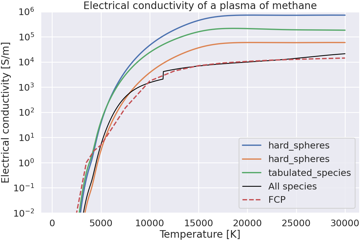
Total running time of the script: (0 minutes 2.945 seconds)