—
Interactive Reaction Path Diagrams for CH₄ plasma chemistry.#
This example uses ipywidgets to create interactive displays of reaction path
diagrams from Cantera simulations.
Inspired by https://cantera.org/3.1/examples/python/kinetics/interactive_path_diagram.html.
Requires: cantera >= 3.0.0, matplotlib >= 2.0, ipywidgets, graphviz, scipy
Import the required libraries.#
import cantera as ct
import graphviz
import matplotlib.pyplot as plt
import numpy as np
from adjustText import adjust_text
from scipy import integrate

from rizer.misc.ct_utils import load_goutier2025_mechanism
from rizer.misc.plt_utils import (
    get_reaction_in_latex,
    get_species_color,
    get_species_in_latex,
    get_text,
    set_mpl_style,
)

set_mpl_style(nb_columns=1)
print(f"Using Cantera version: {ct.__version__}")

# Determine if we're running in a Jupyter Notebook. If so, we can enable the interactive
# diagrams. Otherwise, just draw output for a single set of inputs.
try:
    from IPython.core.getipython import get_ipython

    config = get_ipython()
    if config is None:
        raise ImportError("console")

except (ImportError, AttributeError):
    is_interactive = False
else:
    is_interactive = True

if is_interactive:
    from IPython.display import display
    from ipywidgets import interact, widgets

print(
    "Running in interactive mode"
    if is_interactive
    else "Running in non-interactive mode"
)
Using Cantera version: 4.0.0a2
Running in non-interactive mode
Create the gas object and set the initial conditions.#
# Load the Goutier2025 mechanism.
gas = load_goutier2025_mechanism("gas_with_electronic_excited_states")

# Set the initial temperature, pressure and composition.
gas.TPX = 15_000.0, ct.one_atm, "CH4:1.0"

# Set the residence time for the reactor network.
residence_time = 1e-5  # s

# Create an ideal gas constant pressure reactor and set solver tolerances.
reactor = ct.IdealGasConstPressureReactor(gas, energy="off")
reactor_network = ct.ReactorNet([reactor])
reactor_network.atol = 1e-14
reactor_network.rtol = 1e-14
reactor_network.max_time_step = 1e-8

# Plot options.
xlim = (1e-12, residence_time)

# Wanted species.
wanted_species = "C2H5+"

# Store the reactions and reaction equations.
gas_reactions = gas.reactions()
gas_reaction_equations = gas.reaction_equations()
Store time, pressure, temperature and mole fractions.#
# Store the states in a SolutionArray.
states = ct.SolutionArray(gas, 1, extra={"t": [0.0]})
# Store the number of steps.
steps = 0

# Run the simulation.
while reactor_network.time < residence_time:
    reactor_network.step()
    states.append(gas.state, t=reactor_network.time)
    steps += 1


time = states.t  # type: ignore
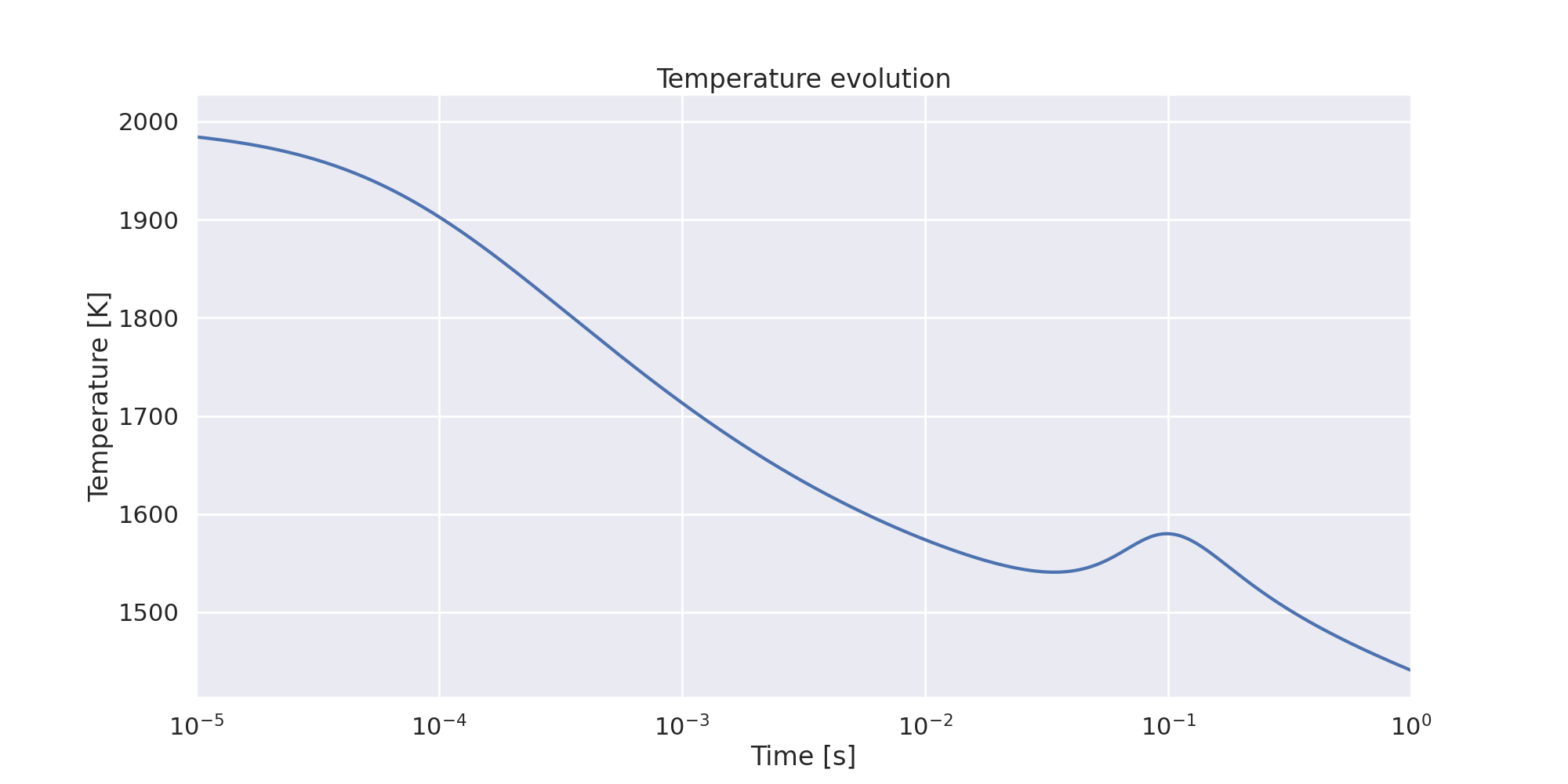
Plot temperature evolution with time.#
fig, ax = plt.subplots()
ax.plot(
    time,
    states.T,
)
ax.set_ylabel("Temperature [K]")
ax.set_title("Temperature evolution")
ax.set_xlabel("Time [s]")
ax.set_xscale("log")
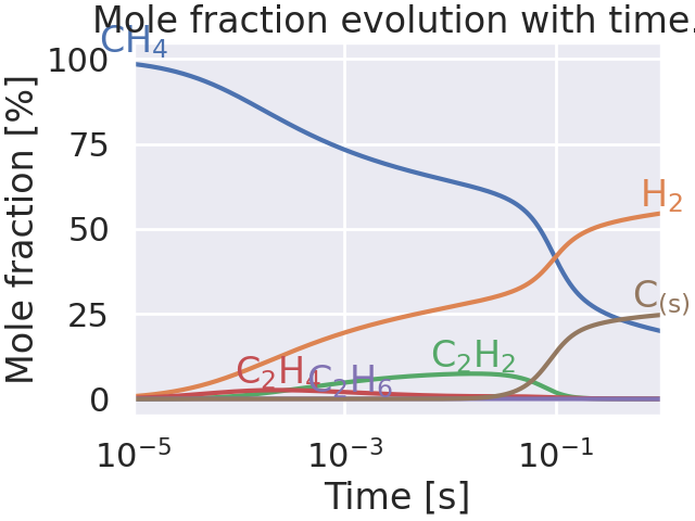
Plot species evolution with time.#
fig, ax = plt.subplots()

species_to_plot = set(["CH4", "H2", "C2H2", "C2H4", "C2H6", "H", wanted_species])
for species in species_to_plot:
    X = states(species).X * 100
    ax.plot(time, X, color=get_species_color(species))

    x = time[np.argmax(X)]
    y = X[np.argmax(X)]
    if x < 1e-11:
        x = 1e-11
        y = X[np.where(time >= 1e-11)[0][0]]

    get_text(
        x,
        y,
        get_species_in_latex(species),
        ax=ax,
        color=get_species_color(species),
    )

ax.set_xlabel("Time [s]")
ax.set_ylabel("Mole fraction [%]")
ax.set_title("Mole fraction evolution with time.")
ax.set_xscale("log")
ax.set_yscale("log")
ax.set_xlim(xlim)
ax.set_ylim(1e-9, 100)
(1e-09, 100)
Interactive reaction path diagram.#
When executed as a Jupyter Notebook, the plotted time step, threshold and element can be changed using the slider provided by IPyWidgets.
def plot_reaction_path_diagrams(plot_step, threshold, details, element):
    P = states.P[plot_step]
    T = states.T[plot_step]
    X = states.X[plot_step]
    gas.TPX = T, P, X

    diagram = ct.ReactionPathDiagram(gas, element)
    diagram.threshold = threshold
    diagram.title = f"time = {time[plot_step]:.2g} s"

    diagram.show_details = details
    if is_interactive:
        graph = graphviz.Source(diagram.get_dot())
        display(graph)
    else:
        graph = graphviz.Source(diagram.get_dot(), format="svg")
        return graph


if is_interactive:
    interact(
        plot_reaction_path_diagrams,
        plot_step=widgets.IntSlider(value=100, min=0, max=steps - 1, step=10),
        threshold=widgets.FloatSlider(value=0.1, min=0.001, max=0.4, step=0.01),
        details=widgets.ToggleButton(),
        element=widgets.Dropdown(
            options=gas.element_names,
            value="C",
            description="Element",
            disabled=False,
        ),
    )
    diagram = ""
else:
    # For non-interactive use, just draw the diagram for a specified time step.
    diagram = plot_reaction_path_diagrams(
        plot_step=520, threshold=0.1, details=False, element="C"
    )


class PlotGraphviz:
    # See https://stackoverflow.com/questions/65008861/capturing-graphviz-figures-in-sphinx-gallery.
    def __init__(self, dot_string):
        self.dot_string = dot_string

    def _repr_html_(self):
        return graphviz.Source(self.dot_string)._repr_image_svg_xml()


PlotGraphviz(str(diagram))
<__main__.PlotGraphviz object at 0x7f49556cf8c0>
Interactive plot of instantaneous fluxes.#
Find reactions containing the species of interest, meaning that the species is either a product or a reactant of the reaction.
wanted_species_stoichiometry = np.zeros_like(gas_reactions, dtype=float)
for i, r in enumerate(gas_reactions):
    wanted_species_stoichiometry[i] = r.products.get(
        wanted_species, 0
    ) - r.reactants.get(wanted_species, 0)
wanted_species_reaction_indices = wanted_species_stoichiometry.nonzero()[0]
Net rates of progress of reactions containing interested species.#
The following cell calculates net rates of progress of reactions containing the species of interest and stores them.
# Some reactions may appear twice, one for forward and one for backward reaction,
# like "e- + CH4 => e- + e- + CH4+" and "e- + e- + CH4+ => e- + CH4"
# Get the pairs of indices of each reaction.
reaction_indices_pairs = []

for i, reaction in enumerate(gas_reactions):
    if " <=> " in reaction.equation:
        continue
    for j, reaction_2 in enumerate(gas_reactions):
        if " <=> " in reaction_2.equation:
            continue
        if (j, i) in reaction_indices_pairs:
            continue

        reactants_2, products_2 = reaction_2.equation.split(" => ")
        reverse_reaction_from_2 = " => ".join([products_2, reactants_2])
        if reaction.equation == reverse_reaction_from_2:
            reaction_indices_pairs.append((i, j))
            break

# Check that the number of reactions computed is correct.
nb_reactions_computed = 2 * len(reaction_indices_pairs) + len(
    [r for r in gas_reactions if " <=> " in r.equation]
)
assert len(gas_reaction_equations) == nb_reactions_computed

# Compute the production rates of the wanted species.
production_rates_wanted_species = (
    states.net_rates_of_progress  # type: ignore
    * wanted_species_stoichiometry
)


for i, j in reaction_indices_pairs:
    # Update the net rates of progress of the forward reactions.
    production_rates_wanted_species[:, i] += production_rates_wanted_species[:, j]
    # Set the net rates of progress of the backward reactions to 0.
    production_rates_wanted_species[:, j] = 0.0

# Net rates of progress [kmol/m^3/s]
wanted_species_production_rates_array = (
    production_rates_wanted_species[:, wanted_species_reaction_indices]  # type: ignore
)


# To avoid the complexity of reading the graph, for each reaction:
# - If the extremum of the net rate of progress is positive,
#   and the wanted species is a product, do nothing.
# - If the extremum of the net rate of progress is positive,
#   and the wanted species is a reactant, inverse the equation.
# - If the extremum of the net rate of progress is negative,
#   and the wanted species is a product, inverse the equation
# - If the extremum of the net rate of progress is negative,
#   and the wanted species is a reactant, do nothing.
#
# To understand the logic, see the following example:
# The reaction "C2H5+ + e- <=> C2H4 + H" is implemented via:
#   (1) C2H5+ + e- => C2H4  + H
#   (2) C2H4  + H  => C2H5+ + e-
# The formation of C2H5+ is given by:
#   d[C2H5+]/dt = - k1 [C2H5+] [e-] + k2 [C2H4] [H]
# With `net_rates_of_progress`, the following quantities are computed:
#   (1) k1 [C2H5+] [e-]
#   (2) k2 [C2H4] [H]
# `wanted_species_stoichiometry` is giving '-1' for (1) and '+1' for (2).
# Thus, `net_rates_of_progress * wanted_species_stoichiometry` gives the
# expected result.
# If we instead choose to implement "C2H4 + H <=> C2H5+ + e" via:
#   (1') C2H4  + H  => C2H5+ + e-
#   (2') C2H5+ + e- => C2H4  + H
# Then, d[C2H5+]/dt = - k2' [C2H5+] [e-] + k1' [C2H4] [H]
# And since k1'=k2 and k2'=k1, we still get the same production rate,
# but the reading is simpler (with the logic above).

for i, production_rate in enumerate(wanted_species_production_rates_array.T):
    production = production_rate[np.argmax(np.abs(production_rate))]

    reaction_idx = wanted_species_reaction_indices[i]

    if production > 0:
        if wanted_species in gas_reactions[reaction_idx].products:
            continue
    else:
        if wanted_species in gas_reactions[reaction_idx].reactants:
            continue
    equation = gas_reaction_equations[reaction_idx]
    equation = equation.replace(" => ", " <=> ")
    reactants, products = equation.split(" <=> ")
    equation = " <=> ".join([products, reactants])
    gas_reaction_equations[reaction_idx] = equation
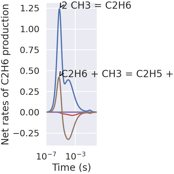
Create the instantaneous flux plot. When executed as a Jupyter Notebook, the threshold for annotating of reaction strings can be changed using the slider provided by IPyWidgets.
total_wanted_species_production_rates = np.sum(
    wanted_species_production_rates_array, axis=1
)


def plot_instantaneous_fluxes(annotation_cutoff):
    fig, ax = plt.subplots()
    texts = []
    for i, wanted_species_production_rate in enumerate(
        wanted_species_production_rates_array.T
    ):
        peak_index = np.argmax(np.abs(wanted_species_production_rate))
        peak_time = time[peak_index]
        peak_wanted_species_production = wanted_species_production_rate[peak_index]
        reaction_string = gas_reaction_equations[wanted_species_reaction_indices[i]]

        ax.plot(time, wanted_species_production_rate)

        if abs(peak_wanted_species_production) > annotation_cutoff:
            texts.append(
                get_text(
                    x=peak_time,
                    y=peak_wanted_species_production,
                    text=get_reaction_in_latex(
                        reaction_string, force_double_arrow=True
                    ),
                    ax=ax,
                )
            )

    ax.plot(time, total_wanted_species_production_rates, "k--")
    if abs(total_wanted_species_production_rates[-1]) > annotation_cutoff:
        texts.append(
            get_text(
                x=time[-1],
                y=total_wanted_species_production_rates[-1],
                text=f"Total {get_species_in_latex(wanted_species)} production",
                ax=ax,
                color="k",
            )
        )

    ax.set_xlabel("Time (s)")
    ax.set_ylabel(f"Net rates of {get_species_in_latex(wanted_species)}")
    ax.set_xscale("log")
    ax.set_xlim(xlim)
    adjust_text(texts, avoid_self=False)
    plt.show()


if is_interactive:
    interact(
        plot_instantaneous_fluxes,
        annotation_cutoff=widgets.FloatSlider(value=0.1, min=0.1, max=200, steps=100),
    )
else:
    plot_instantaneous_fluxes(annotation_cutoff=0.1)
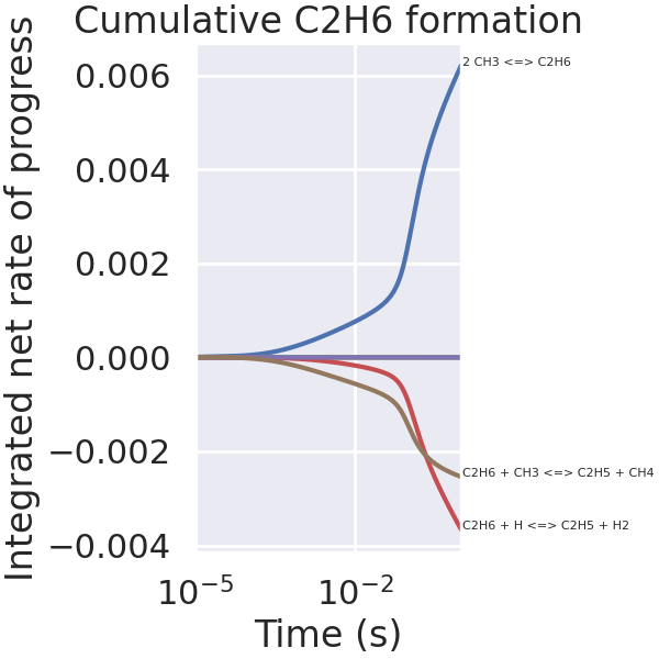
Interactive plot of integrated fluxes.#
When executed as a Jupyter Notebook, the threshold for annotating of reaction strings can be changed using the slider provided by iPyWidgets.
# Integrate fluxes over time.
integrated_fluxes = integrate.cumulative_trapezoid(
    wanted_species_production_rates_array,
    time,
    axis=0,
    initial=0,
)

# Sum of all integrated fluxes.
total_integrated_fluxes = np.sum(integrated_fluxes, axis=1)


def plot_integrated_fluxes(integrated_fluxes, annotation_cutoff):
    fig, ax = plt.subplots()

    texts = []

    for i, wanted_species_production in enumerate(integrated_fluxes.T):
        total_wanted_species_production = wanted_species_production[-1]

        equation = gas_reaction_equations[wanted_species_reaction_indices[i]]

        ax.plot(time, wanted_species_production)

        if abs(total_wanted_species_production) > annotation_cutoff:
            texts.append(
                get_text(
                    x=float(1e-4),
                    y=float(total_wanted_species_production),
                    text=get_reaction_in_latex(equation, force_double_arrow=True),
                    ax=ax,
                )
            )

    ax.plot(time, total_integrated_fluxes, "k--")
    if abs(total_wanted_species_production) > annotation_cutoff:
        texts.append(
            get_text(
                x=float(1e-4),
                y=float(total_integrated_fluxes[-1]),
                text=f"Total integrated flux: {total_integrated_fluxes[-1]:.2g}",
                ax=ax,
                color="k",
            )
        )

    ax.set_xlabel("Time (s)")
    ax.set_ylabel("Integrated net rates of progress")
    ax.set_title(
        f"Cumulative {get_species_in_latex(wanted_species)} formation/decomposition"
    )
    ax.set_xscale("log")
    ax.set_xlim(xlim)
    adjust_text(texts, avoid_self=False)
    plt.show()


if is_interactive:
    interact(
        plot_integrated_fluxes,
        annotation_cutoff=widgets.FloatLogSlider(
            value=1e-5, min=-8, max=-4, base=10, step=0.1
        ),
        integrated_fluxes=widgets.fixed(integrated_fluxes),
    )
else:
    plot_integrated_fluxes(integrated_fluxes=integrated_fluxes, annotation_cutoff=1e-5)
Total running time of the script: (0 minutes 5.174 seconds)