—
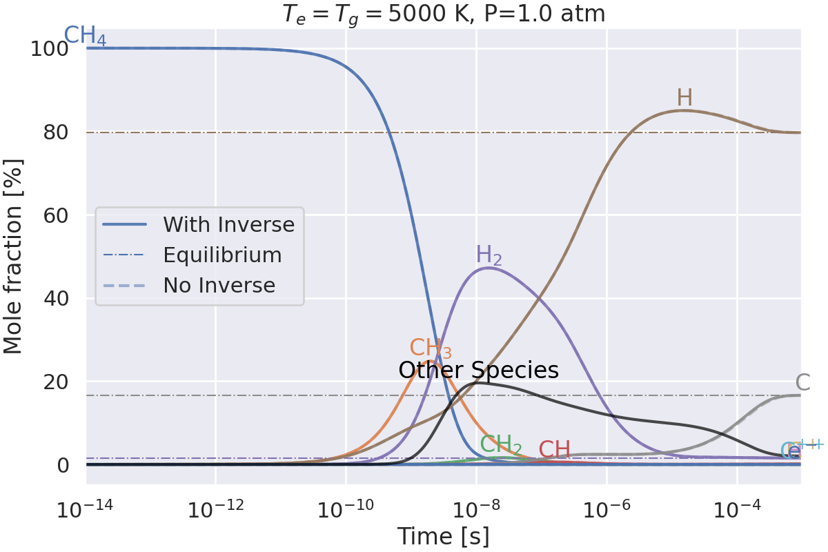
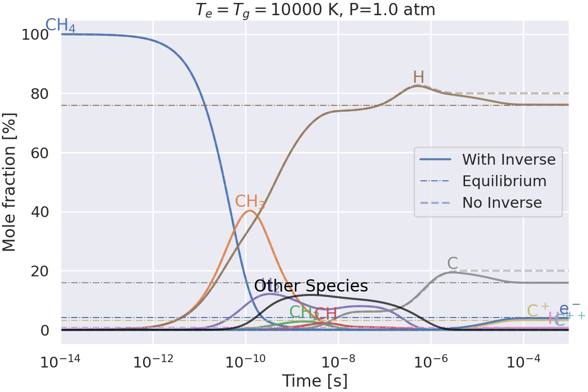
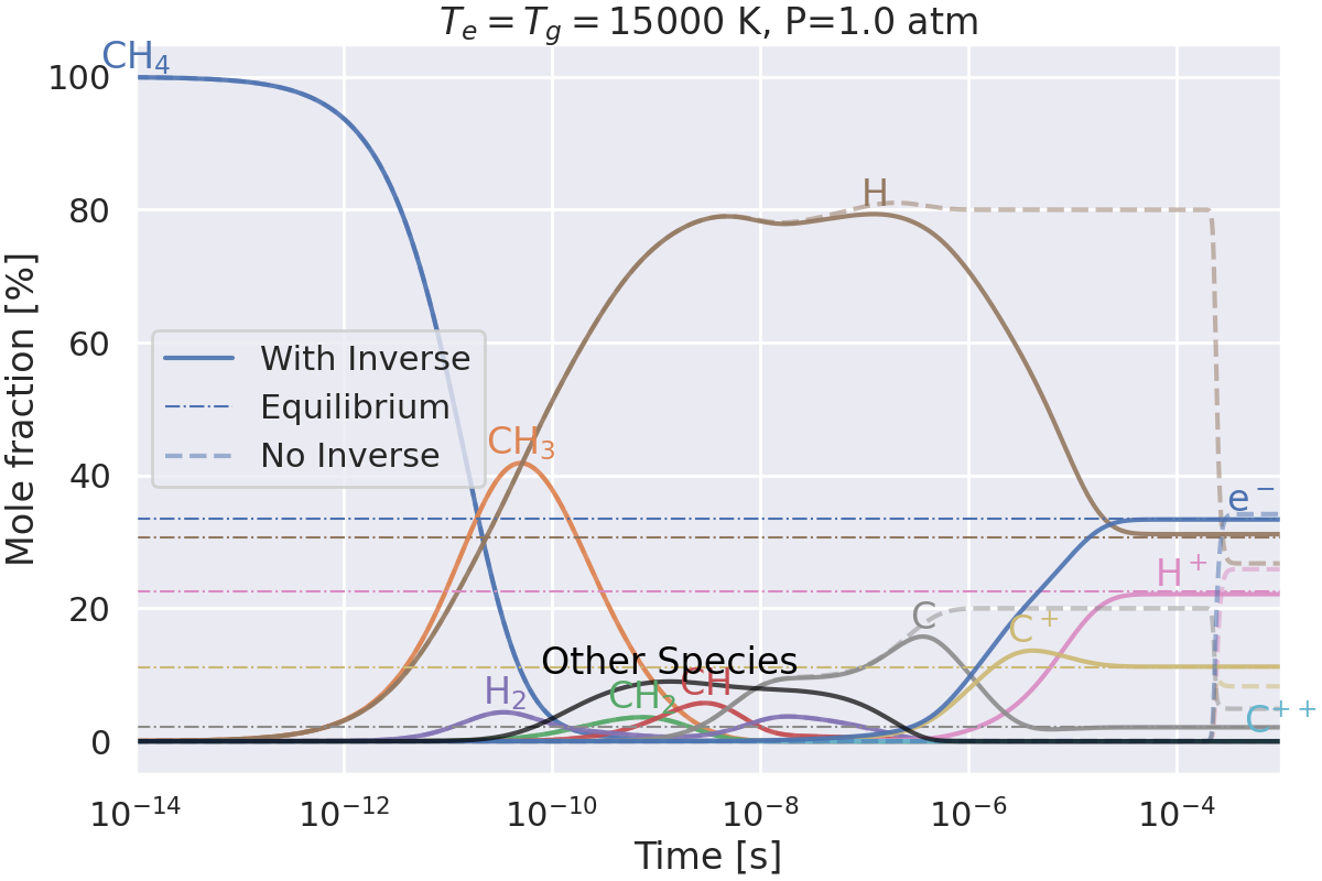
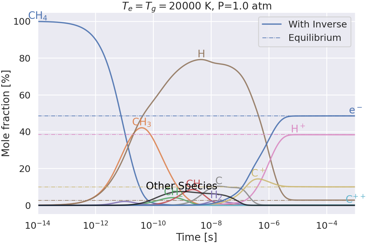
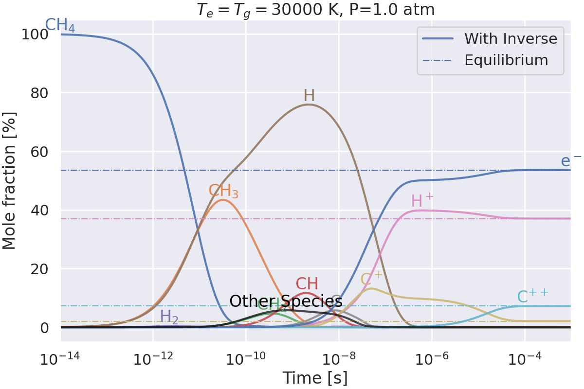
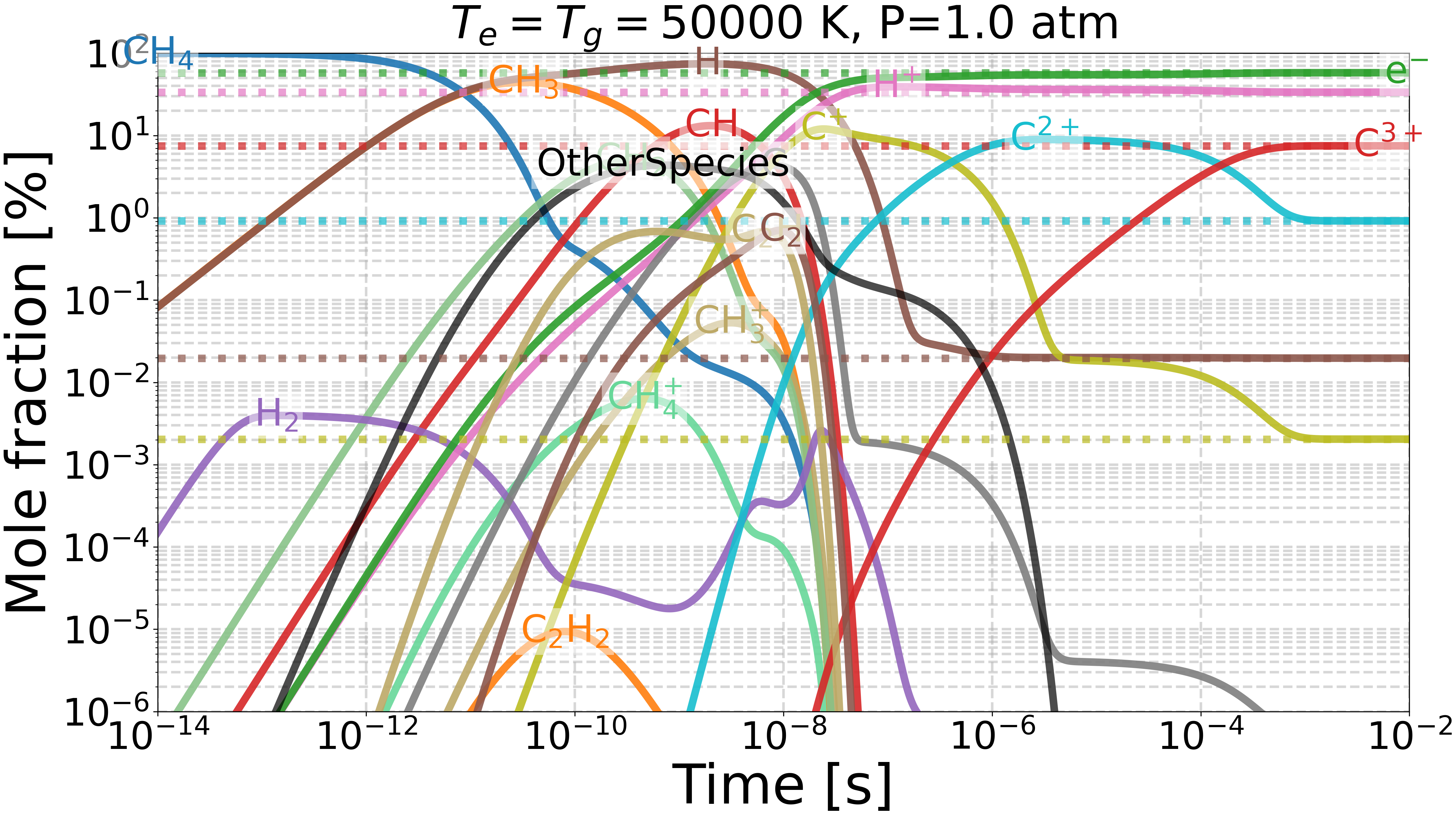
Do we get the same equilibrium with and without inverse reactions?#
This example checks if the equilibrium of two mechanisms is the same:
one with inverse reactions,
one without inverse reactions.
Key formula used for reverse rate constant calculation:
\[k_b = \frac{k_f}{K_{eq}}\]
where:
\(k_b\): backward rate constant
\(k_f\): forward rate constant
\(K_{eq}\): equilibrium constant
The equilibrium constant is computed from Gibbs free energy:
\[K_{eq} = \exp\left(-\frac{\Delta G}{R T}\right)\]
where:
\(\Delta G\): Gibbs free energy change
\(R\): universal gas constant
\(T\): temperature
For two-temperature plasma reactions, in equilibrium, the electron temperature is equal to the gas temperature, and the rate constant is computed using the above formula.
# This is an option for the online documentation, so that each image is displayed separately.
# sphinx_gallery_multi_image = "single"
# sphinx_gallery_thumbnail_number = 9
Import the required libraries.#
from dataclasses import dataclass, field

import cantera as ct
import matplotlib.pyplot as plt
import numpy as np
from adjustText import adjust_text

from rizer.misc.ct_utils import load_goutier2025_mechanism
from rizer.misc.plt_utils import (
    get_species_color,
    get_species_in_latex,
    get_text,
    set_mpl_style,
)
from rizer.misc.utils import get_path_to_data

set_mpl_style(nb_columns=1)
Define mechanisms and parameters.#
gas_no_inverse = ct.Solution(
    get_path_to_data(
        "mechanisms",
        "Goutier2025",
        "builder",
        "CH4_to_C2H2_forward_reactions.yaml",
    ),
    name="gas",
)
gas_arrhenius_rates = load_goutier2025_mechanism("gas_with_electronic_excited_states")
# gas_druyvesteyn_rates = load_goutier2025_mechanism(
#     "gas_druyvesteyn_with_electronic_excited_states"
# )


# Temperatures in Kelvin.
# For the mechanism with inverse reactions, we can go up to 50000 K,
# because the equilibrium is reached and the results are reliable.
temperatures_with_inverse = np.array(
    [
        1000,
        2000,
        5000,
        10000,
        15000,
        20000,
        30000,
        40000,
        50000,
    ]
)
# For the mechanism without inverse reactions, we cannot go higher than 15000 K,
# because the equilibrium is not reached and the results are not reliable.
temperatures_no_inverse = temperatures_with_inverse[temperatures_with_inverse < 15000]
# Pressure in Pascals.
P = ct.one_atm
# Initial mole fraction (here, we start with pure methane).
X_0 = "CH4:1"

# Species to plot (colors are assigned via get_species_color for consistency across examples).
species_to_plot = [
    "CH4",
    "CH4+",
    "CH3",
    "CH3+",
    "CH2",
    "CH",
    "H2",
    "H",
    "H(n=2)",
    "H(n=3)",
    "H(n=4)",
    "H+",
    "C",
    "C(1D)",
    "C(1S)",
    "C(5So)",
    "C+",
    "C++",
    "C+++",
    "e-",
    "C2H2",
    "C2H",
    "C2",
]

# Parameters for the reactor network.
simulation_time = 1e-2  # Simulation time in seconds
rtol = 1e-11  # Relative tolerance for the reactor network
max_steps = 100_000  # Maximum steps for the reactor network
max_time_step = 1e-5  # Maximum time step for the reactor network
Define the state groups for the different mechanisms.#
@dataclass
class StateGroup:
    solution: ct.Solution
    temperatures: np.ndarray
    linestyle: str
    linewidth: float
    states: list[ct.SolutionArray] = field(default_factory=list)


no_inverse = StateGroup(
    solution=gas_no_inverse,
    temperatures=temperatures_no_inverse,
    linestyle="--",
    linewidth=5,
)
with_arrhenius_rates = StateGroup(
    solution=gas_arrhenius_rates,
    temperatures=temperatures_with_inverse,
    linestyle="-",
    linewidth=6,
)
# with_druyvesteyn_rates = StateGroup(
#     solution=gas_druyvesteyn_rates,
#     temperatures=temperatures_with_inverse,
#     linestyle="-.",
#     linewidth=5,
# )


all_states: list[StateGroup] = [
    no_inverse,
    with_arrhenius_rates,
    # with_druyvesteyn_rates,
]
Compute equilibrium and time evolution for each mechanism and each temperature.#
# Compute the equilibrium for the mechanism with inverse reactions.
states_eq = ct.SolutionArray(gas_arrhenius_rates, shape=temperatures_with_inverse.shape)
states_eq.TPX = temperatures_with_inverse, P, X_0
states_eq.equilibrate("TP")

# Compute the time evolution for each mechanism and each temperature.
for state_group in all_states:
    print(f"Running equilibrium for {state_group.solution.name} mechanism")

    for T in state_group.temperatures:
        print(f"Running equilibrium for T={T} K")

        # Initialize the reactor network for the current temperature.
        state_group.solution.TPX = T, P, X_0
        r1 = ct.IdealGasConstPressureReactor(state_group.solution, energy="off")
        sim = ct.ReactorNet([r1])
        sim.rtol = rtol  # Set relative tolerance for the reactor network.
        sim.max_time_step = max_time_step
        sim.reinitialize()

        # Store the states in a SolutionArray.
        states = ct.SolutionArray(state_group.solution, 1, extra={"t": [0.0]})

        i = 0

        while sim.time < simulation_time:
            # Advance the reactor network by one step.
            sim.step()
            # Append the current state to the SolutionArray.
            states.append(state_group.solution.state, t=sim.time)  # type: ignore

            i += 1

            if i % 1000 == 0:
                print(f"{sim.time:.2e} / {simulation_time:.2e}")

        state_group.states.append(states)
Running equilibrium for gas mechanism
Running equilibrium for T=1000 K
9.89e-03 / 1.00e-02
Running equilibrium for T=2000 K
9.69e-05 / 1.00e-02
2.09e-03 / 1.00e-02
Running equilibrium for T=5000 K
5.89e-08 / 1.00e-02
2.57e-06 / 1.00e-02
1.66e-03 / 1.00e-02
Running equilibrium for T=10000 K
4.45e-09 / 1.00e-02
3.71e-07 / 1.00e-02
6.05e-06 / 1.00e-02
6.88e-03 / 1.00e-02
Running equilibrium for gas_with_electronic_excited_states mechanism
Running equilibrium for T=1000 K
9.88e-03 / 1.00e-02
Running equilibrium for T=2000 K
9.53e-05 / 1.00e-02
2.47e-03 / 1.00e-02
Running equilibrium for T=5000 K
6.60e-08 / 1.00e-02
3.22e-06 / 1.00e-02
1.54e-03 / 1.00e-02
Running equilibrium for T=10000 K
4.71e-09 / 1.00e-02
3.75e-07 / 1.00e-02
3.32e-06 / 1.00e-02
7.09e-05 / 1.00e-02
8.64e-03 / 1.00e-02
Running equilibrium for T=15000 K
1.84e-09 / 1.00e-02
8.79e-08 / 1.00e-02
5.60e-07 / 1.00e-02
6.26e-06 / 1.00e-02
6.74e-03 / 1.00e-02
Running equilibrium for T=20000 K
9.95e-10 / 1.00e-02
3.58e-08 / 1.00e-02
1.79e-07 / 1.00e-02
2.03e-04 / 1.00e-02
9.80e-03 / 1.00e-02
Running equilibrium for T=30000 K
3.79e-10 / 1.00e-02
9.92e-09 / 1.00e-02
7.94e-08 / 1.00e-02
8.81e-05 / 1.00e-02
8.76e-03 / 1.00e-02
Running equilibrium for T=40000 K
1.88e-10 / 1.00e-02
3.06e-09 / 1.00e-02
2.93e-08 / 1.00e-02
6.86e-06 / 1.00e-02
6.23e-03 / 1.00e-02
Running equilibrium for T=50000 K
6.10e-11 / 1.00e-02
1.70e-09 / 1.00e-02
5.80e-09 / 1.00e-02
3.85e-08 / 1.00e-02
3.33e-04 / 1.00e-02
9.38e-03 / 1.00e-02
Plotting the results.#
for i, T in enumerate(temperatures_with_inverse):
    print(f"Plotting results for T={T} K")

    fig, ax = plt.subplots()

    # Storage for the maximum mole fraction with the corresponding time
    # of each species across all states.
    # The third value is the value in the equilibrium.
    max_fractions: dict[str, tuple[float, float, float]] = {
        species: (
            0.0,  # Maximum mole fraction
            0.0,  # Corresponding time
            0.0,  # Value in the equilibrium
        )
        for species in species_to_plot
    }
    max_fractions["Other Species"] = (0.0, 0.0, 0.0)

    for j, state_group in enumerate(all_states):
        if i >= len(state_group.temperatures):
            continue

        states = state_group.states[i]
        other_species = np.ones_like(states.t) * 100.0  # type: ignore

        for species in species_to_plot:
            if species not in state_group.solution.species_names:
                continue

            # Plot the time evolution of the mole fraction.
            x = states.t  # type: ignore
            y = states(species).X * 100
            other_species -= y[:, 0]
            color = get_species_color(species)
            ax.plot(
                x,
                y,
                linestyle=state_group.linestyle,
                linewidth=state_group.linewidth,
                alpha=0.9,
                color=color,
            )
            # Add the species name at the maximum point, with the same color as the line.
            max_x = x[y.argmax()]
            if max_x < 1e-14:
                max_x = 1e-14
            max_y = y.max()
            # Update the maximum fraction and corresponding time for the species.
            if j != 0:
                # For the mechanism without inverse reactions, we cannot trust the results,
                # so we skip the update of the maximum fraction.
                if max_y > max_fractions[species][0]:
                    max_fractions[species] = (
                        max_y,
                        max_x,
                        states_eq[i](species).X[-1] * 100,
                    )

        # Plot the remaining species as "Other Species"
        ax.plot(
            states.t,  # type: ignore
            other_species,
            linestyle=state_group.linestyle,
            linewidth=state_group.linewidth,
            alpha=0.7,
            color="black",
        )
        # Add the species name at the maximum point, with the same color as the line.
        max_x = states.t[np.argmax(other_species)]  # type: ignore
        if max_x < 1e-14:
            max_x = 1e-14
        max_y = np.max(other_species)
        # Update the maximum fraction and corresponding time for "Other Species".
        if max_y > max_fractions["Other Species"][0]:
            max_fractions["Other Species"] = (max_y, max_x, 0.0)

    # Plot the equilibrium values as horizontal lines.
    for species in species_to_plot:
        if species not in states_eq.species_names:
            continue
        y_eq = states_eq[i](species).X * 100
        color = get_species_color(species)
        ax.hlines(
            y=y_eq,
            xmin=1e-14,
            xmax=simulation_time,
            linestyle=":",
            color=color,
            alpha=0.7,
            linewidth=6,
        )

    # Add a text label for the species.
    # For species present in the equilibrium (with a mole fraction above 1e-5),
    # add it at the end of the simulation.
    # For other species, add it at the maximum of all the states (unless their
    # maximum mole fraction is below 1e-5, in which case we skip them).
    texts = []
    for species, (max_y, max_x, y_eq) in max_fractions.items():
        if max_y < 1e-5 and species != "Other Species":
            continue  # Skip species with a maximum mole fraction below 1e-5.

        if y_eq > 1e-5:
            x = simulation_time
            y = y_eq
        else:
            x = max_x
            y = max_y

        text = get_text(
            x,
            y,
            get_species_in_latex(species)
            if species != "Other Species"
            else "Other Species",
            ax=ax,
            color=get_species_color(species) if species != "Other Species" else "black",
        )
        texts.append(text)

    ax.set_title(f"$T_e=T_g={T}$ K, P={int(P / ct.one_atm):.1f} atm")
    ax.set_xlabel("Time [s]")
    ax.set_xlim(left=1e-14, right=simulation_time)
    ax.set_xscale("log")
    ax.set_ylabel("Mole fraction [%]")
    ax.set_ylim(bottom=1e-5, top=100)
    ax.set_yscale("log")

    adjust_text(
        texts,
        avoid_self=False,
        expand=(
            1.2,
            2,
        ),  # expand text bounding boxes by 1.2 fold in x direction and 2 fold in y direction
        arrowprops=dict(
            arrowstyle="->", color="red"
        ),  # ensure the labeling is clear by adding arrows
    )

    plt.show()
Plotting results for T=1000 K
/home/runner/micromamba/envs/DEVELOP/lib/python3.14/site-packages/adjustText/__init__.py:422: UserWarning: constrained_layout not applied because axes sizes collapsed to zero.  Try making figure larger or Axes decorations smaller.
  ax.figure.draw_without_rendering()
Plotting results for T=2000 K
Plotting results for T=5000 K
Plotting results for T=10000 K
Plotting results for T=15000 K
Plotting results for T=20000 K
Plotting results for T=30000 K
Plotting results for T=40000 K
Plotting results for T=50000 K
Total running time of the script: (0 minutes 16.974 seconds)