—
Analysis of Thor4 generator data.#
Analysis of Thor4 generator data with different resistance models (Rompe-Weizel, Vlastos, Braginskii). Data comes from run 143 of the Thor4 generator, in test T176.
The circuit solved is the following:
    ┌-------------L1--------------┐
 ↑  │                             │    ↑
 │  │                             L2   │
u_c C                             │   u_mes
 │  │                             R    │
 │  │                             │    │
    ┖-----------------------------┘
The resistance R can be one the following models:
Import the required libraries.#
import matplotlib.pyplot as plt
import numpy as np

from rizer.electric_circuit.rllc_circuit import RLLC_Circuit
from rizer.electric_circuit.variable_resistance_models import (
    BraginskiiResistance,
    ConstantResistance,
    RompeWeizelResistance,
    VlastosResistance,
)
from rizer.misc.plt_utils import set_mpl_style
from rizer.misc.utils import get_path_to_data

set_mpl_style(nb_columns=1)
Loading the data.#
path_to_data = get_path_to_data(
    "experiments", "Thor4_T176", "run143_capacity_discharge.csv"
)
time, voltage, voltage_std, current, current_std = np.genfromtxt(
    path_to_data, skip_header=6, unpack=True, delimiter=";"
)
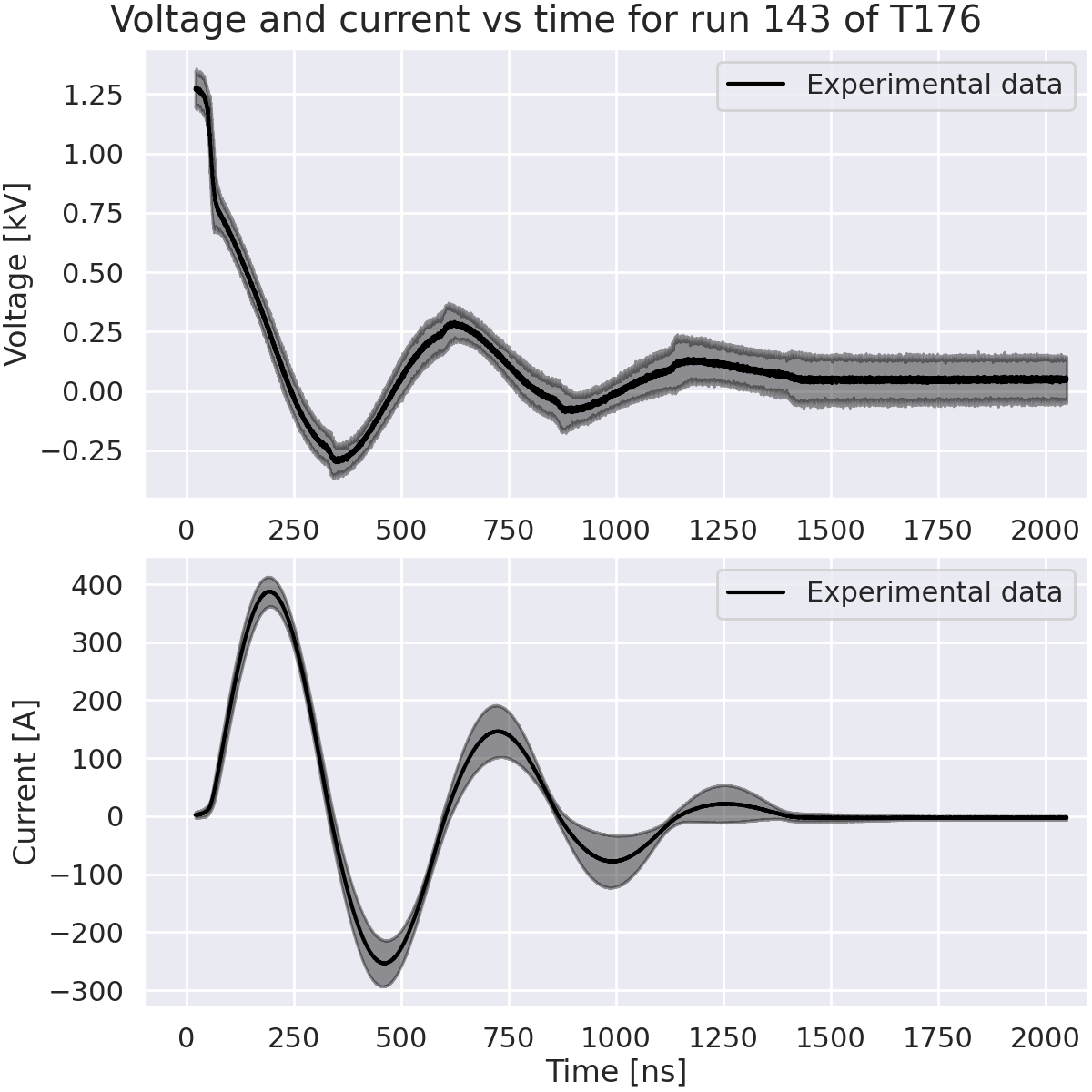
Plot voltage and current vs time.#
fig, axes = plt.subplots(2, 1, figsize=(12, 12), layout="constrained")
assert isinstance(axes, np.ndarray)
xlims = (-100, 2100)
axes[0].plot(time * 1e9, voltage / 1e3, label="Experimental data", color="black")
axes[0].set_ylabel("Voltage [kV]")
axes[0].set_xlim(xlims)
axes[0].legend()
axes[0].fill_between(
    time * 1e9,
    (voltage - 2 * voltage_std) / 1e3,  # 2 standard deviation for 95% uncertainty.
    (voltage + 2 * voltage_std) / 1e3,  # 2 standard deviation for 95% uncertainty.
    alpha=0.4,
    color="black",
)
axes[1].plot(time * 1e9, current, label="Experimental data", color="black")
axes[1].set_ylabel("Current [A]")
axes[1].set_xlim(xlims)
axes[1].legend()
axes[1].set_xlabel("Time [ns]")
axes[1].fill_between(
    time * 1e9,
    current - 2 * current_std,  # 2 standard deviation for 95% uncertainty.
    current + 2 * current_std,  # 2 standard deviation for 95% uncertainty.
    alpha=0.4,
    color="black",
)

fig.suptitle("Voltage and current vs time for run 143 of T176")
plt.show()
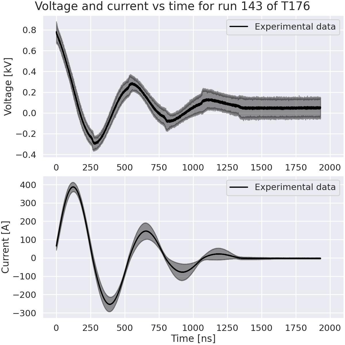
Zoom on capacitor discharge.#
We will zoom on the capacitor discharge to better see the voltage and current evolution. We will only keep the data between 70 ns and 2000 ns.
low_cutoff = 70e-9  # s
high_cutoff = 2000e-9  # s
mask = (low_cutoff < time) & (time < high_cutoff)
time_exp = time[mask]
time_exp -= time_exp[0]  # Start at 0
voltage_exp = voltage[mask]
current_exp = current[mask]
voltage_std_exp = voltage_std[mask]
current_std_exp = current_std[mask]

fig, axes = plt.subplots(2, 1, figsize=(12, 12), layout="constrained")
assert isinstance(axes, np.ndarray)
axes[0].plot(
    time_exp * 1e9, voltage_exp / 1e3, label="Experimental data", color="black"
)
axes[0].fill_between(
    time_exp * 1e9,
    (voltage_exp - 2 * voltage_std_exp)
    / 1e3,  # 2 standard deviation for 95% uncertainty.
    (voltage_exp + 2 * voltage_std_exp)
    / 1e3,  # 2 standard deviation for 95% uncertainty.
    alpha=0.4,
    color="black",
)
axes[0].set_ylabel("Voltage [kV]")
axes[0].legend()
axes[0].set_xlim(xlims)
axes[1].plot(time_exp * 1e9, current_exp, label="Experimental data", color="black")
axes[1].fill_between(
    time_exp * 1e9,
    current_exp - 2 * current_std_exp,  # 2 standard deviation for 95% uncertainty.
    current_exp + 2 * current_std_exp,  # 2 standard deviation for 95% uncertainty.
    alpha=0.4,
    color="black",
)
axes[1].set_ylabel("Current [A]")
axes[1].set_xlabel("Time [ns]")
axes[1].legend()
axes[1].set_xlim(xlims)
fig.suptitle("Voltage and current vs time for run 143 of T176")
plt.show()
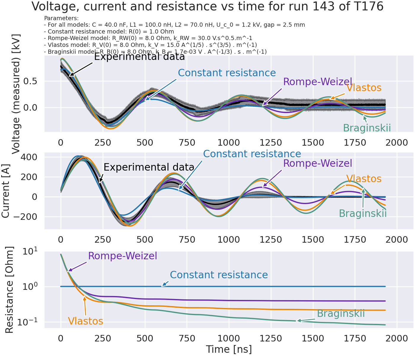
Plot resistance model with various RLLC models#
Recalling that the circuit solved is the following:
    ┌-------------L1--------------┐
 ↑  │                             │    ↑
 │  │                             L2   │
u_c C                             │   u_mes
 │  │                             R    │
 │  │                             │    │
    ┖-----------------------------┘
# -- Parameters for the circuit -- #
C = 40e-9 # F, Capacitance.
L1 = 100e-9 # H, Inductance 1.
L2 = 70e-9 # H, Inductance 2.
I_0 = current_exp[0] # A, initial current measured in the experiment.
u_mes_0 = voltage_exp[0] # V, initial voltage measured in the experiment.
u_L1_0 = np.gradient(current_exp, time_exp)[0] * L1 # V, initial voltage on L1.
U_c_0 = u_mes_0 + u_L1_0 # 782 + 384 = 1166 V
# U_c_0 = 1.1e3 # V, initial voltage on the capacitor.
# -- Parameters for the models -- #
gap = 2.5e-3 # m
# Constant resistance model
R0_C = 1 # Ohm
# Rompe-Weizel model
R0_RW = 8 # Ohm
k_RW = 30 # V.s^0.5.m^-1
# Vlastos model
R0_V = 8 # Ohm
k_V = 15 # A^(1/5) . s^(3/5) . m^(-1).
# Braginskii model
R0_B = 8 # Ohm
k_B = 1.7e-3 # V . A^(-1/3) . s . m^(-1).
# -- Models -- #
# Constant resistance model
ConstantResistance_RLLC = ConstantResistance()
rllc_constant = RLLC_Circuit(
C, L1, L2, R0_C, I_0, U_c_0, R_model=ConstantResistance_RLLC
)
i_num_constant, _, u_num_constant, R_num_constant = rllc_constant.solve(time_exp)
# Rompe-Weizel model
RompeWeizelResistance_RLLC = RompeWeizelResistance(gap, k_RW)
rllc_RW = RLLC_Circuit(C, L1, L2, R0_RW, I_0, U_c_0, R_model=RompeWeizelResistance_RLLC)
i_num_RW, _, u_num_RW, R_num_RW = rllc_RW.solve(time_exp)
# Vlastos model
VlastosResistance_RLLC = VlastosResistance(gap, k_V)
rllc_Vlastos = RLLC_Circuit(C, L1, L2, R0_V, I_0, U_c_0, R_model=VlastosResistance_RLLC)
i_num_Vlastos, _, u_num_Vlastos, R_num_Vlastos = rllc_Vlastos.solve(time_exp)
# Braginskii model
BraginskiiResistance_RLLC = BraginskiiResistance(gap, k_B)
rllc_Braginskii = RLLC_Circuit(
C, L1, L2, R0_B, I_0, U_c_0, R_model=BraginskiiResistance_RLLC
)
i_num_Braginskii, _, u_num_Braginskii, R_num_Braginskii = rllc_Braginskii.solve(
time_exp
)
# ---- Plot the voltage, current and resistance vs time. ---- #
# -- Figure, axes and title -- #
fig, axes = plt.subplots(3, 1, figsize=(14, 12), layout="constrained")
assert isinstance(axes, np.ndarray)
fig.suptitle("Voltage, current and resistance vs time for run 143 of T176")
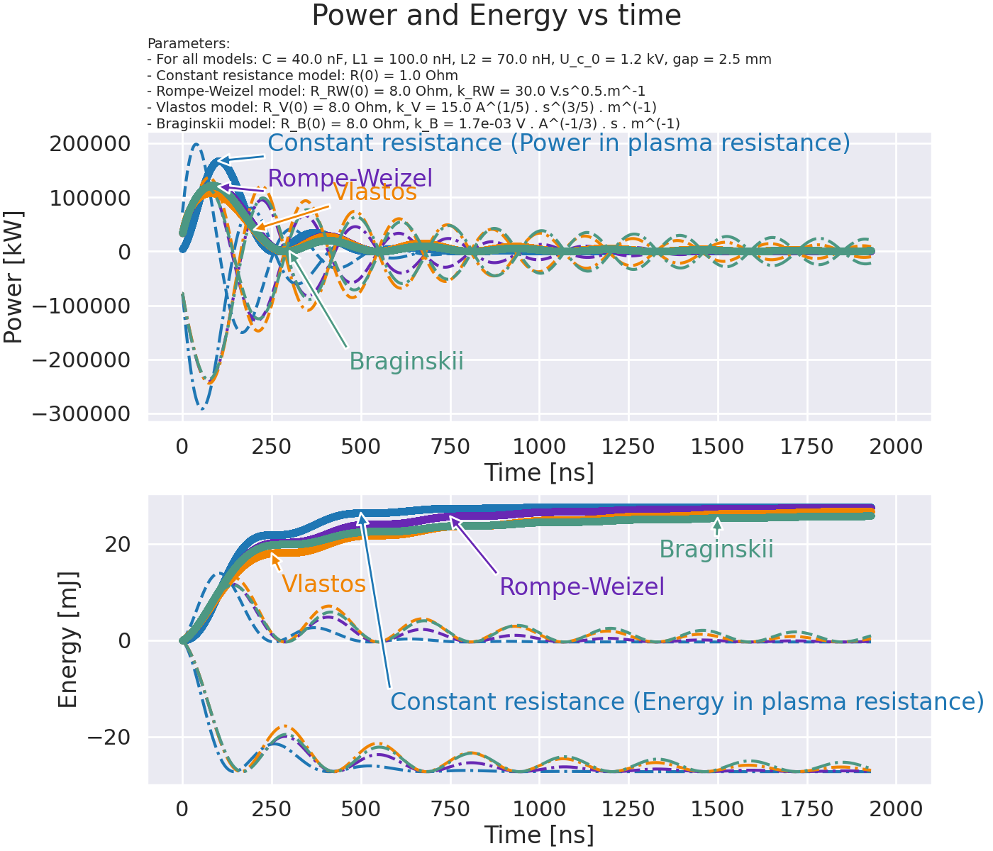
title = (
"Parameters:\n"
f"- For all models: C = {C * 1e9:.1f} nF, L1 = {L1 * 1e9:.1f} nH, L2 = {L2 * 1e9:.1f} nH, "
f"U_c_0 = {U_c_0 / 1e3:.1f} kV, gap = {gap * 1e3:.1f} mm\n"
f"- Constant resistance model: R(0) = {R0_C:.1f} Ohm\n"
f"- Rompe-Weizel model: R_RW(0) = {R0_RW:.1f} Ohm, k_RW = {k_RW:.1f} V.s^0.5.m^-1\n"
f"- Vlastos model: R_V(0) = {R0_V:.1f} Ohm, k_V = {k_V:.1f} A^(1/5) . s^(3/5) . m^(-1)\n"
f"- Braginskii model: R_B(0) = {R0_B:.1f} Ohm, k_B = {k_B:.1e} V . A^(-1/3) . s . m^(-1)"
)
axes[0].set_title(title, fontsize=14, pad=3, loc="left")
# -- Voltage -- #
# Plot options
axes[0].set_ylabel("Voltage (measured) [kV]")
axes[0].set_xlim(xlims)
# Parameters for the annotations.
plot_params = {
"data": [voltage_exp, u_num_constant, u_num_RW, u_num_Vlastos, u_num_Braginskii],
"label": [
"Experimental data",
"Constant resistance",
"Rompe-Weizel",
"Vlastos",
"Braginskii",
],
"x_arrow": [ # Time in ns for the x position of the arrow.
50,
500,
1200,
1600,
1800,
],
"xy_offset": [ # Offset for the annotation (in points).
(60, 40),
(80, 60),
(50, 50),
(40, 20),
(-50, -40),
],
"color": ["black", "#1f77b4", "#6828B4", "#F08400", "#4C9883"],
}
for key in plot_params:
assert len(plot_params[key]) == len(plot_params["data"])
# Plot
for i in range(len(plot_params["data"])):
data = plot_params["data"][i]
x_arrow = plot_params["x_arrow"]
color = plot_params["color"][i]
time = np.argmin(np.abs(time_exp - x_arrow[i] * 1e-9))
axes[0].plot(time_exp * 1e9, data / 1e3, color=color)
axes[0].annotate(
plot_params["label"][i],
(time_exp[time] * 1e9, data[time] / 1e3),
xytext=plot_params["xy_offset"][i],
textcoords="offset points",
color=color,
arrowprops=dict(facecolor=color),
)
# Also plot the experimental data standard deviation.
axes[0].fill_between(
time_exp * 1e9,
(voltage_exp - 2 * voltage_std_exp) / 1e3,
(voltage_exp + 2 * voltage_std_exp) / 1e3,
alpha=0.4,
color="black",
)
# -- Current -- #
# Plot options
axes[1].set_ylabel("Current [A]")
axes[1].set_xlim(xlims)
# Parameters for the annotations.
plot_params = {
"data": [current_exp, i_num_constant, i_num_RW, i_num_Vlastos, i_num_Braginskii],
"label": [
"Experimental data",
"Constant resistance",
"Rompe-Weizel",
"Vlastos",
"Braginskii",
],
"x_arrow": [ # Time in ns for the x position of the arrow.
230,
700,
1200,
1600,
1800,
],
"xy_offset": [ # Offset for the annotation (in points).
(10, 30),
(60, 80),
(50, 50),
(40, 30),
(-60, -70),
],
"color": ["black", "#1f77b4", "#6828B4", "#F08400", "#4C9883"],
}
for key in plot_params:
assert len(plot_params[key]) == len(plot_params["data"])
# Plot
for i in range(len(plot_params["data"])):
data = plot_params["data"][i]
x_arrow = plot_params["x_arrow"]
color = plot_params["color"][i]
time = np.argmin(np.abs(time_exp - x_arrow[i] * 1e-9))
axes[1].plot(time_exp * 1e9, data, color=color)
axes[1].annotate(
plot_params["label"][i],
(time_exp[time] * 1e9, data[time]),
xytext=plot_params["xy_offset"][i],
textcoords="offset points",
color=color,
arrowprops=dict(facecolor=color),
)
# Also plot the experimental data standard deviation.
axes[1].fill_between(
time_exp * 1e9,
current_exp - 2 * current_std_exp,
current_exp + 2 * current_std_exp,
alpha=0.4,
color="black",
)
# -- Resistance -- #
# Plot options
axes[2].set_ylabel("Resistance [Ohm]")
axes[2].set_xlim(xlims)
axes[2].set_yscale("log")
axes[2].set_xlabel("Time [ns]")
# Parameters for the annotations.
plot_params = {
"data": [R_num_constant, R_num_RW, R_num_Vlastos, R_num_Braginskii],
"label": ["Constant resistance", "Rompe-Weizel", "Vlastos", "Braginskii"],
"x_arrow": [ # Time in ns for the x position of the arrow.
600,
40,
140,
1400,
],
"xy_offset": [ # Offset for the annotation (in points).
(20, 20),
(50, 30),
(-40, -70),
(50, 10),
],
"color": ["#1f77b4", "#6828B4", "#F08400", "#4C9883"],
}
for key in plot_params:
assert len(plot_params[key]) == len(plot_params["data"])
# Plot
for i in range(len(plot_params["data"])):
data = plot_params["data"][i]
x_arrow = plot_params["x_arrow"]
color = plot_params["color"][i]
time = np.argmin(np.abs(time_exp - x_arrow[i] * 1e-9))
axes[2].plot(time_exp * 1e9, data, color=color)
axes[2].annotate(
plot_params["label"][i],
(time_exp[time] * 1e9, data[time]),
xytext=plot_params["xy_offset"][i],
textcoords="offset points",
color=color,
arrowprops=dict(facecolor=color),
)
plt.show()
Compute power and energy for the different models.#
# Compute powers.
R_power_constant, L_power_constant, C_power_constant = rllc_constant.get_powers()
R_power_RW, L_power_RW, C_power_RW = rllc_RW.get_powers()
R_power_Vlastos, L_power_Vlastos, C_power_Vlastos = rllc_Vlastos.get_powers()
R_power_Braginskii, L_power_Braginskii, C_power_Braginskii = (
    rllc_Braginskii.get_powers()
)
# Compute energies.
R_energy_constant, L_energy_constant, C_energy_constant = rllc_constant.get_energies()
R_energy_RW, L_energy_RW, C_energy_RW = rllc_RW.get_energies()
R_energy_Vlastos, L_energy_Vlastos, C_energy_Vlastos = rllc_Vlastos.get_energies()
R_energy_Braginskii, L_energy_Braginskii, C_energy_Braginskii = (
    rllc_Braginskii.get_energies()
)

# -- Plot power and energy vs time. -- #
fig, axes = plt.subplots(2, 1, figsize=(14, 12), layout="constrained")
assert isinstance(axes, np.ndarray)
fig.suptitle("Power and Energy vs time")
axes[0].set_title(title, fontsize=14, pad=3, loc="left")

# First, plot power.
# Parameters for the annotations.
plot_params = {
    "data": [
        [R_power_constant, L_power_constant, C_power_constant],
        [R_power_RW, L_power_RW, C_power_RW],
        [R_power_Vlastos, L_power_Vlastos, C_power_Vlastos],
        [R_power_Braginskii, L_power_Braginskii, C_power_Braginskii],
    ],
    "label": [
        "Constant resistance (Power in plasma resistance)",
        "Rompe-Weizel",
        "Vlastos",
        "Braginskii",
    ],
    "x_arrow": [  # Time in ns for the x position of the arrow.
        100,
        100,
        200,
        300,
    ],
    "xy_offset": [  # Offset for the annotation (in points).
        (50, 10),
        (50, 0),
        (80, 30),
        (60, -120),
    ],
    "color": [
        "#1f77b4",
        "#6828B4",
        "#F08400",
        "#4C9883",
    ],
}

for key in plot_params:
    assert len(plot_params[key]) == len(plot_params["data"])

# Plot
for i in range(len(plot_params["data"])):
    datas = plot_params["data"][i]
    data_R = datas[0]
    data_L = datas[1]
    data_C = datas[2]

    x_arrow = plot_params["x_arrow"]
    color = plot_params["color"][i]

    time = np.argmin(np.abs(time_exp - x_arrow[i] * 1e-9))
    axes[0].plot(time_exp * 1e9, data_R, ".", color=color)
    axes[0].plot(time_exp * 1e9, data_L, "--", color=color)
    axes[0].plot(time_exp * 1e9, data_C, "-.", color=color)

    axes[0].annotate(
        plot_params["label"][i],
        (time_exp[time] * 1e9, data_R[time]),
        xytext=plot_params["xy_offset"][i],
        textcoords="offset points",
        color=color,
        arrowprops=dict(facecolor=color),
    )
axes[0].set_ylabel("Power [kW]")
axes[0].set_xlabel("Time [ns]")
axes[0].set_xlim(xlims)

# Second, plot energy.
# Parameters for the annotations.
plot_params = {
    "data": [
        [R_energy_constant, L_energy_constant, C_energy_constant],
        [R_energy_RW, L_energy_RW, C_energy_RW],
        [R_energy_Vlastos, L_energy_Vlastos, C_energy_Vlastos],
        [R_energy_Braginskii, L_energy_Braginskii, C_energy_Braginskii],
    ],
    "label": [
        "Constant resistance (Energy in plasma resistance)",
        "Rompe-Weizel",
        "Vlastos",
        "Braginskii",
    ],
    "x_arrow": [  # Time in ns for the x position of the arrow.
        500,
        750,
        250,
        1500,
    ],
    "xy_offset": [  # Offset for the annotation (in points).
        (30, -200),
        (50, -80),
        (10, -40),
        (-60, -40),
    ],
    "color": [
        "#1f77b4",
        "#6828B4",
        "#F08400",
        "#4C9883",
    ],
}

for key in plot_params:
    assert len(plot_params[key]) == len(plot_params["data"])

# Plot
for i in range(len(plot_params["data"])):
    datas = plot_params["data"][i]
    data_R = datas[0] * 1e3  # Convert to mJ
    data_L = datas[1] * 1e3  # Convert to mJ
    data_C = datas[2] * 1e3  # Convert to mJ

    x_arrow = plot_params["x_arrow"]
    color = plot_params["color"][i]

    time = np.argmin(np.abs(time_exp - x_arrow[i] * 1e-9))
    axes[1].plot(time_exp * 1e9, data_R, ".", color=color)
    axes[1].plot(time_exp * 1e9, data_C, "-.", color=color)
    axes[1].plot(time_exp * 1e9, data_L, "--", color=color)

    axes[1].annotate(
        plot_params["label"][i],
        (time_exp[time] * 1e9, data_R[time]),
        xytext=plot_params["xy_offset"][i],
        textcoords="offset points",
        color=color,
        arrowprops=dict(facecolor=color),
    )

axes[1].set_ylabel("Energy [mJ]")
axes[1].set_xlabel("Time [ns]")
axes[1].set_xlim(xlims)
(-100.0, 2100.0)
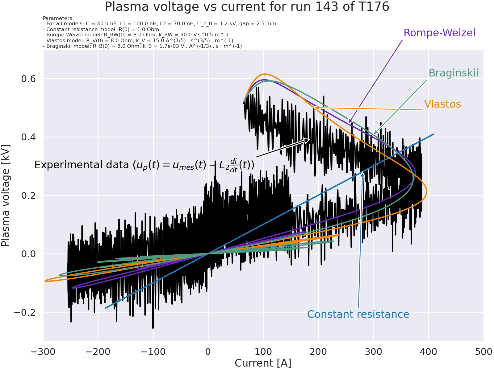
Plot plasma voltage versus current for the different models#
# Compute experimental plasma voltage.
plasma_voltage = voltage_exp - L2 * np.gradient(current_exp, time_exp)
fig, axes = plt.subplots(1, 1, figsize=(16, 12), layout="constrained")
fig.suptitle("Plasma voltage vs current for run 143 of T176")
axes.set_title(title, fontsize=12, pad=3, loc="left")

# Voltage vs current.
axes.set_xlabel("Current [A]")
axes.set_xlim(-300, 500)
axes.set_ylabel("Plasma voltage [kV]")
axes.set_ylim(-0.3, 0.7)

# Parameters for the annotations.
n_exp = 300
n_constant = 400
n_RW = 600
n_Vlastos = 400
n_Braginskii = 800

plot_params = {
    "x_data": [current_exp, i_num_constant, i_num_RW, i_num_Vlastos, i_num_Braginskii],
    "y_data": [
        plasma_voltage,
        R_num_constant * i_num_constant,
        R_num_RW * i_num_RW,
        R_num_Vlastos * i_num_Vlastos,
        R_num_Braginskii * i_num_Braginskii,
    ],
    "label": [
        r"Experimental data ($u_p(t)=u_{mes}(t)-L_2 \frac{di}{dt}(t)$)",
        "Constant resistance",
        "Rompe-Weizel",
        "Vlastos",
        "Braginskii",
    ],
    "xy_arrow": [
        (current_exp[n_exp], plasma_voltage[n_exp] / 1e3),
        (
            i_num_constant[n_constant],
            R_num_constant[n_constant] * i_num_constant[n_constant] / 1e3,
        ),
        (i_num_RW[n_RW], R_num_RW[n_RW] * i_num_RW[n_RW] / 1e3),
        (
            i_num_Vlastos[n_Vlastos],
            R_num_Vlastos[n_Vlastos] * i_num_Vlastos[n_Vlastos] / 1e3,
        ),
        (
            i_num_Braginskii[n_Braginskii],
            R_num_Braginskii[n_Braginskii] * i_num_Braginskii[n_Braginskii] / 1e3,
        ),
    ],  # Current in A for the x position of the arrow, Voltage in kV for the y position of the arrow.
    "xy_offset": [
        (current_exp[n_exp] - 500, plasma_voltage[n_exp] / 1e3 - 0.1),
        (
            i_num_constant[n_constant] - 100,
            R_num_constant[n_constant] * i_num_constant[n_constant] / 1e3 - 0.5,
        ),
        (i_num_RW[n_RW] + 100, R_num_RW[n_RW] * i_num_RW[n_RW] / 1e3 + 0.3),
        (
            i_num_Vlastos[n_Vlastos] + 200,
            R_num_Vlastos[n_Vlastos] * i_num_Vlastos[n_Vlastos] / 1e3,
        ),
        (
            i_num_Braginskii[n_Braginskii] + 100,
            R_num_Braginskii[n_Braginskii] * i_num_Braginskii[n_Braginskii] / 1e3 + 0.2,
        ),
    ],  # Current in A for the x position of the text, Voltage in kV for the y position of the text.
    "color": ["black", "#1f77b4", "#6828B4", "#F08400", "#4C9883"],
}

for key in plot_params:
    assert len(plot_params[key]) == len(plot_params["y_data"])

# Plot.
for i in range(len(plot_params["y_data"])):
    x_data = plot_params["x_data"][i]
    y_data = plot_params["y_data"][i] / 1e3
    color = plot_params["color"][i]

    axes.plot(x_data, y_data, color=color)
    axes.annotate(
        plot_params["label"][i],
        plot_params["xy_arrow"][i],
        xytext=plot_params["xy_offset"][i],
        color=color,
        arrowprops=dict(facecolor=color),
    )

plt.show()
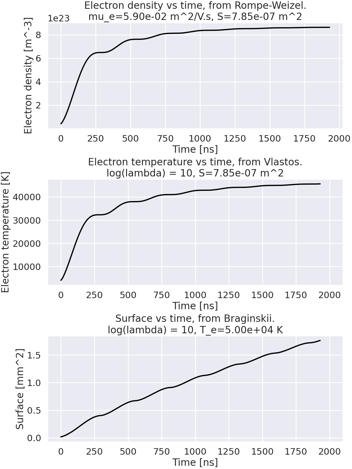
Plot electron density, electron temperature and surface for each model.#
mu_e = 0.059  # electron mobility in m^2/V.s (Air at atmospheric pressure and room temperature)
r_0 = 0.5e-3  # m, radius of the plasma
S = np.pi * r_0**2  # m^2, surface of the plasma
log_lambda = 10  # Coulomb logarithm
n_e = RompeWeizelResistance_RLLC.get_electron_density(mu_e=mu_e, S=S)
T_e = VlastosResistance_RLLC.get_temperature_evolution(log_lambda=log_lambda, S=S)
T_e_RW = 50_000  # K, electron temperature
S_B = BraginskiiResistance_RLLC.get_area_evolution(log_lambda=log_lambda, T_e=T_e_RW)

fig, axes = plt.subplots(3, 1, figsize=(12, 16), layout="constrained")

# Plot the electron density evolution (Rompe-Weizel model).

axes[0].set_title(
    f"Electron density vs time, from Rompe-Weizel.\nmu_e={mu_e:.2e} m^2/V.s, S={S:.2e} m^2",
)
axes[0].set_ylabel("Electron density [m^-3]")
axes[0].set_xlabel("Time [ns]")
axes[0].plot(time_exp * 1e9, n_e, label="Electron density", color="black")


# Plot the temperature evolution (Vlastos model).

axes[1].set_title(
    f"Electron temperature vs time, from Vlastos.\nlog(lambda) = {log_lambda}, S={S:.2e} m^2",
)
axes[1].set_ylabel("Electron temperature [K]")
axes[1].set_xlabel("Time [ns]")
axes[1].set_xlim(xlims)
axes[1].plot(time_exp * 1e9, T_e, label="Electron temperature", color="black")


# Plot the surface evolution (Branginskii model).

axes[2].set_title(
    f"Surface vs time, from Braginskii.\nlog(lambda) = {log_lambda}, T_e={T_e_RW:.2e} K",
)
axes[2].set_ylabel("Surface [mm^2]")
axes[2].set_xlabel("Time [ns]")
axes[2].set_xlim(xlims)
axes[2].plot(time_exp * 1e9, S_B * 1e6, label="Surface", color="black")

plt.show()
Total running time of the script: (0 minutes 5.006 seconds)