—
Cross sections and reaction rate constant for the ionisation of CH₄ by electrons.#
This example shows how to load cross section data for the ionisation of CH₄ by electrons from different databases, plot the cross sections, and compute the reaction rate constant.
The reaction considered is CH₄ + e⁻ -> CH₄⁺ + e⁻ + e⁻.
The cross section data is loaded from the following databases (all available on the LXCat website, except for the Janev database):
Hayashi [Hayashi2010]
IST Lisbonne [ISTLisbonne1995]
Morgan [Morgan1992]
Song Bouwman [SongBouwman2021]
Janev [Janev2002]
Note#
The reaction rate constant is computed from the cross section data, assuming that electrons follow a Maxwellian distribution, using the following formula:
where:
\(k(T)\) is the reaction rate constant,
\(\sigma(E)\) is the cross section,
\(v(E)\) is the electron velocity,
\(f(E)\) is the electron distribution function.
Then, the reaction rate constant is fitted to a modified Arrhenius expression, through a least-squares fit. The modified Arrhenius expression is given by:
where:
\(A\) is the pre-exponential factor,
\(b\) is the temperature exponent,
\(E_a\) is the activation energy (here, in Kelvin).
Import the required libraries.#
import matplotlib.pyplot as plt
import numpy as np

import rizer.misc.units as u
from rizer.io.lxcat import Collision, LXCat
from rizer.kin.fit_arrhenius import arrhenius_rate, k_fit_arrhenius_lstsq
from rizer.misc.plt_utils import set_mpl_style
from rizer.misc.utils import get_path_to_data
from rizer.plasma.equations import compute_electronic_reaction_rate_constant

set_mpl_style(nb_columns=1)
Load one cross section data and plot it.#
# Load the cross section data from the Song Bouwman database.
lx = LXCat(verbose=False)
lx.read(file=get_path_to_data("kin", "cross_section", "CH4", "SongBouwman.txt"))
['CH4']
Print the data for the CH₄ -> CH₄⁺ reaction.
df: Collision = lx.species["CH4"].collisions["CH4 -> CH4+"]
print(f"Species: {df.species_name}")
print(f"Reaction: {df.reaction}")
print(f"Threshold energy: {df.threshold} eV")
Species: CH4
Reaction: CH4 -> CH4+
Threshold energy: 12.63 eV
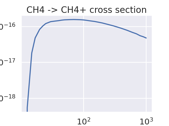
Plot the cross section data.
fig, ax = plt.subplots()
ax.plot(df.energy_eV, df.cross_section_cm2)
ax.set_xlabel("Energy [eV]")
ax.set_ylabel("Cross section [cm²]")
ax.set_title(
    r"Cross section of $\mathrm{CH_4 + e^- \rightarrow CH_4^+ + 2e^-}$ from S. Bouwman"
)
ax.set_xscale("log")
ax.set_xlim(left=1, right=1e4)
ax.set_yscale("log")
plt.show()
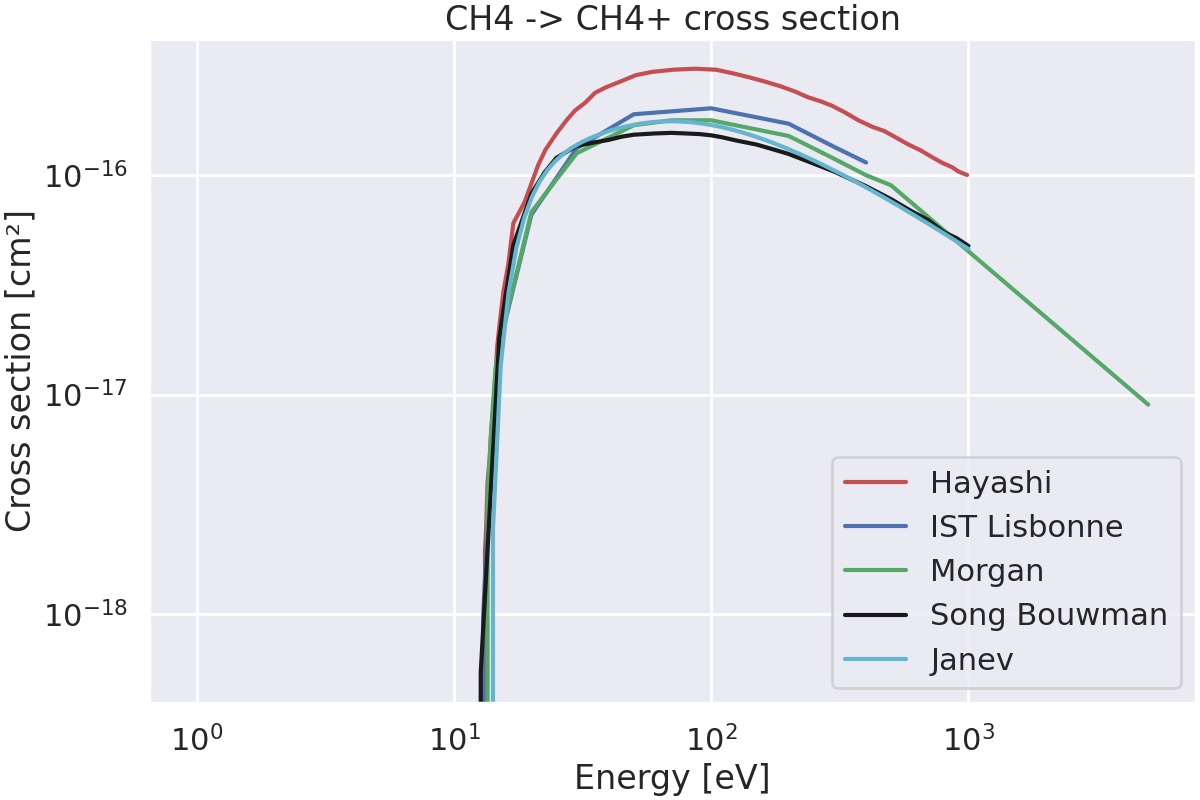
Plot the cross sections from different databases.#
# Dictionary to store the cross section data.
# Key: name of the cross section database
# Value: dictionary with:
#   - reaction: reaction name
#   - color: color for the plot
#   - label: label for the plot
cross_sections_data = {
    "Hayashi.txt": {
        "reaction": "CH4 -> CH4^+",
        "color": "r",
        "label": "Hayashi",
    },
    "ISTLisbonne.txt": {
        "reaction": "CH4 -> CH4+",
        "color": "b",
        "label": "IST Lisbonne",
    },
    "Morgan.txt": {
        "reaction": "CH4 -> CH4^+",
        "color": "g",
        "label": "Morgan",
    },
    "SongBouwman.txt": {
        "reaction": "CH4 -> CH4+",
        "color": "k",
        "label": "Song Bouwman",
    },
    "janev_cross_sections_CH4.txt": {
        "reaction": "CH4 -> CH4^+",
        "color": "c",
        "label": "Janev",
    },
}

# Dictionary to store reactions data.
# Key: reactions name
# Value: dictionary with:
#   key: name of the cross-section database
#   value: Collision object
reactions_to_plot: dict[str, dict[str, Collision]] = {
    "CH4 -> CH4+": {},
}
Plot the cross sections.
fig, ax = plt.subplots()

for file, data_dict in cross_sections_data.items():
    # Load the cross section data.
    lx = LXCat(verbose=False)
    lx.read(file=get_path_to_data("kin", "cross_section", "CH4", file))

    # Look for the reaction of methane ionization (CH4 -> CH4+) in the file.
    df = lx.species["CH4"].collisions[data_dict["reaction"]]

    # Assign the dataframe to the dictionary.
    reactions_to_plot["CH4 -> CH4+"][file] = df

    # Extract the cross section data as numpy arrays.
    energy_eV: np.ndarray = df.energy_eV
    cross_section_cm2: np.ndarray = df.cross_section_cm2

    # Plot the cross section.
    color = data_dict["color"]
    label = data_dict["label"]
    ax.plot(energy_eV, cross_section_cm2, color=color, label=label)

# Set the labels and title.
ax.set_xlabel("Energy [eV]")
ax.set_ylabel("Cross section [cm²]")
ax.set_title(r"Cross section of $\mathrm{CH_4 + e^- \rightarrow CH_4^+ + 2e^-}$")
ax.set_xscale("log")
ax.set_yscale("log")
ax.set_xlim(left=1, right=1e4)
ax.legend(loc="lower right")
plt.show()
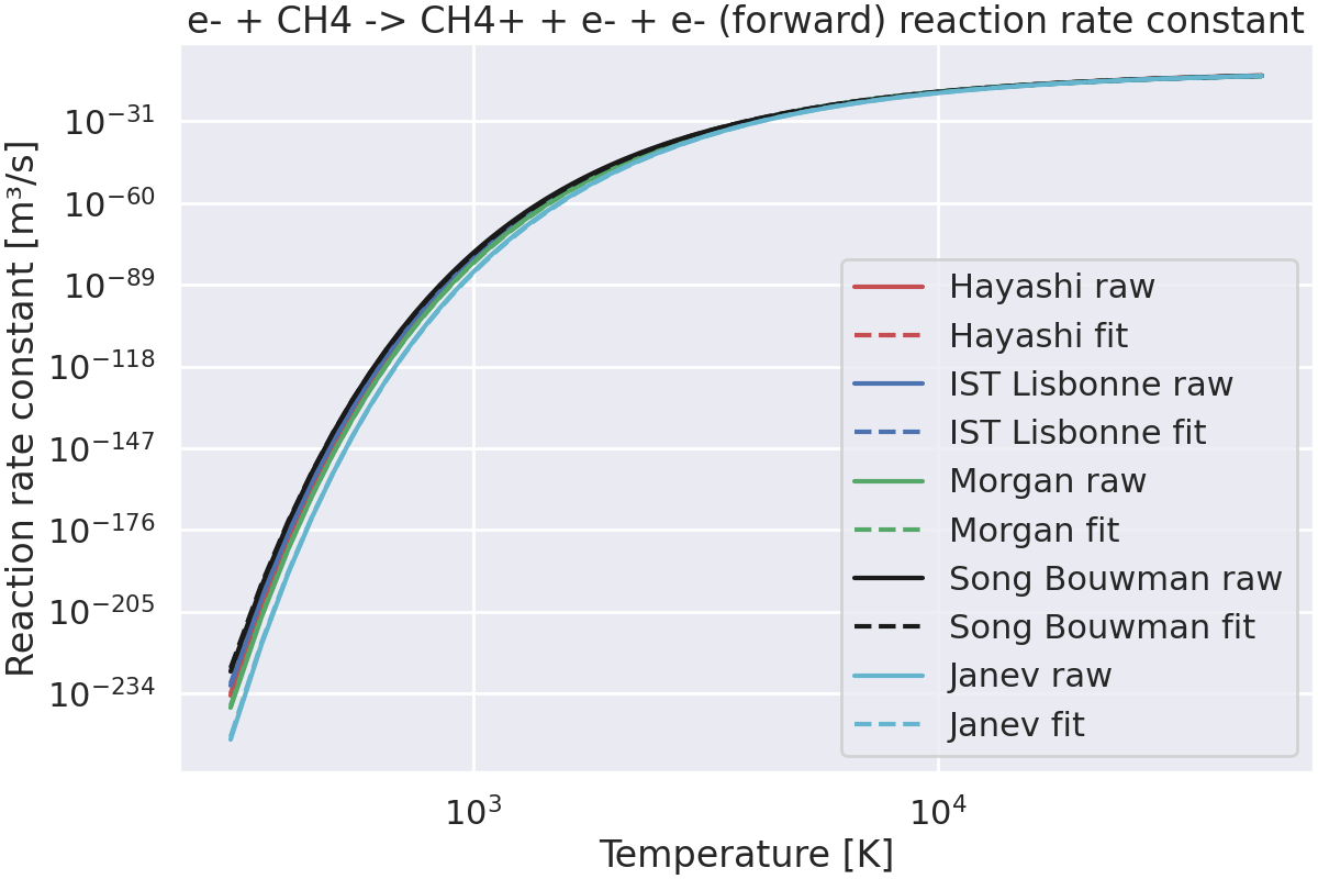
Compute the reaction rate constant.#
# Define the temperatures at which to compute the reaction rate constant.
temperatures = np.linspace(300, 50_000, 1000, dtype=float)
fig, ax1 = plt.subplots()
fig2, ax2 = plt.subplots()
for file, data_dict in cross_sections_data.items():
# Get the reaction data.
df = reactions_to_plot["CH4 -> CH4+"][file]
# Extract the cross section data as numpy arrays,
# and convert the energy to Joules and the cross section to m².
energy_J: np.ndarray = df.energy_eV * u.eV_to_J
cross_section_m2: np.ndarray = df.cross_section_cm2 * 1e-4
# Compute the reaction rate constant, from the cross section.
# NOTE: It is assumed that electrons follow a Maxwellian distribution.
k_forward = np.zeros_like(temperatures) # [m³/s]
for i, T in enumerate(temperatures):
k_forward[i] = compute_electronic_reaction_rate_constant(
T, cross_section_m2, energy_J
)
# Plot the rate constant.
color = data_dict["color"]
label = data_dict["label"]
ax1.plot(temperatures, k_forward, color, label=label + " raw")
# Fit the rate constant to an Arrhenius expression.
# A is in [m³/s], Ea is in [K].
A, b, Ea, _ = k_fit_arrhenius_lstsq(k_forward, temperatures)
k_fit = arrhenius_rate(A, b, Ea, temperatures)
# Print the fit parameters.
print(
f"{file}:\n "
f" A = {A:.2e} m3/s,\tb = {b:.2f},\tEa = {Ea:.2e} K = {Ea * u.K_to_eV:.2f} eV"
)
ax1.plot(temperatures, k_fit, color + "--", label=label + " fit")
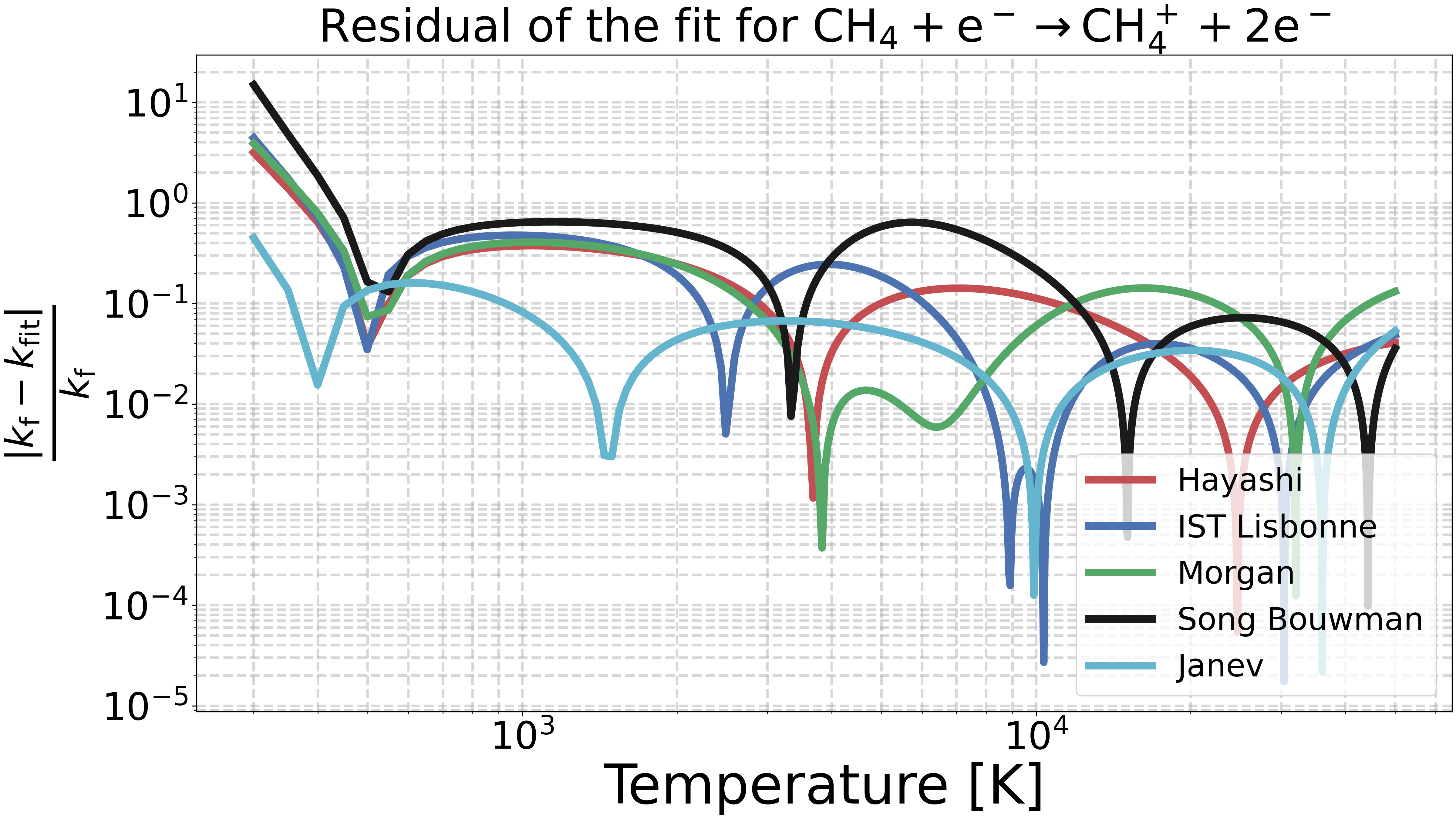
# Plot the residual of the fit.
residual = np.abs(k_forward - k_fit) / k_forward
ax2.plot(temperatures, residual, color, label=label)
# Set the labels and title.
ax1.set_title(
r"Forward reaction rate constant of $\mathrm{CH_4 + e^- \rightarrow CH_4^+ + 2e^-}$"
)
ax1.set_ylabel(r"$k_\text{f}$ [$\mathrm{m^3. s^{-1}}$]")
ax2.set_title(
r"Residual of the fit for $\mathrm{CH_4 + e^- \rightarrow CH_4^+ + 2e^-}$"
)
ax2.set_ylabel(r"$\frac{|k_\text{f} - k_\text{fit}|}{k_\text{f}}$")
for ax in [ax1, ax2]:
ax.legend(fontsize="small", loc="lower right")
ax.set_xlabel("Temperature [K]")
ax.set_xscale("log")
ax.set_yscale("log")
plt.show()
Hayashi.txt:
  A = 7.93e-18 m3/s,    b = 0.78,       Ea = 1.51e+05 K = 13.03 eV
ISTLisbonne.txt:
  A = 9.45e-18 m3/s,    b = 0.73,       Ea = 1.49e+05 K = 12.81 eV
Morgan.txt:
  A = 1.04e-15 m3/s,    b = 0.30,       Ea = 1.55e+05 K = 13.34 eV
SongBouwman.txt:
  A = 2.28e-19 m3/s,    b = 1.08,       Ea = 1.44e+05 K = 12.45 eV
janev_cross_sections_CH4.txt:
  A = 5.68e-18 m3/s,    b = 0.81,       Ea = 1.60e+05 K = 13.80 eV
Total running time of the script: (0 minutes 3.013 seconds)