—

Rempart Mechanism Validation.

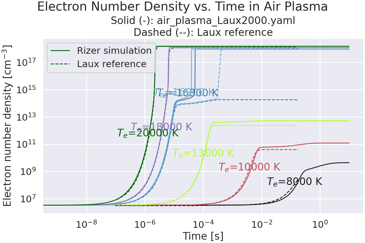
Validation case of Rizer code, as well as plasma air mechanism with Laux Rempart Project reference case.

Case: Two-temperature air plasma with ionization mechanisms from the Rempart Project.

• Constant Gas Temperature: 2000 K

• Constant Gas Pressure: 1 atm

• Initial Electron Number Density: 3.3e6 \(cm^{-3}\)

• Initial Mole Fraction of Air: O2=21%/N2=79%

• Electron Temperatures: from 8000 to 20,0000 K

Comparison with the Laux reference case ([LauxLecture]), with the evolution of electron number density.

Notes

There are two references for the ionization mechanisms in the Rempart Project.

The first one ([Laux2000]) is the original paper by Christophe Laux, while the second one ([LauxLecture]) is a plasma lecture by Christophe Laux. In the original paper, there are 38 reactions (including backward reactions for electronic reactions), and the electron temperature range is from 8000 to 18000 K. In the lecture, there are 40 reactions (but not backward reactions), and the electron temperature range is from 8000 to 20000 K.

Reactions in the present mechanism come from [Laux2000]. The last 2 reactions are added from [LauxLecture].

Tags: kinetics plasma Rempart air validation

Import the required libraries.

import cantera as ct
import matplotlib.pyplot as plt
import numpy as np
import scipy.integrate  # type: ignore
import seaborn as sns
from spy.misc.arrays import logspace  # type: ignore # Spark Python package

from rizer.misc.utils import get_path_to_data
from rizer.plasma.reactor import PlasmaExtension, PlasmaReactorOde, u

sns.set_theme("poster")

Load data from Laux’ lecture [LauxLecture].

# Validation case of C.O. Laux Two-temperature model.
electron_temperatures_K = [8000, 10000, 13000, 16800, 16900, 18000, 20000]
data_laux: list[
    tuple[np.ndarray, np.ndarray]
] = []  # List of tuples with time and electron number density.
for T_e in electron_temperatures_K:
    file = get_path_to_data("papers", "LauxLecture2023", f"{T_e}K.csv")
    time, ne = np.genfromtxt(file, delimiter=",", unpack=True, skip_header=3)
    data_laux.append((time, ne))

# Convert the electron temperatures from Kelvin to eV.
electron_temperatures_eV = np.array(electron_temperatures_K, dtype=float) * u.K_to_eV

Parameters for the simulation.

# Initial condition.
P = ct.one_atm
T0 = 2000  # K
N0_cm3 = (P / u.k_b / T0) * 1e-6  # Initial gas density, cm^-3
n_e_0 = 3.3e6  # Initial electron density, cm^-3
x_e_0 = n_e_0 / N0_cm3  # mole fraction

# Calculation parameters.
t_start = 1e-9  # s
t_end = 10  # s
N_POINTS_STORED = 10000  # Number of points stored in the SolutionArray.
t_array = logspace(t_start, t_end, N_POINTS_STORED)

Create the plasma mechanism and extension objects.

# Define the paths to the plasma mechanism
plasma_mechanism = get_path_to_data("mechanisms", "air_plasma_Laux2000.yaml")
# Load the plasma Solution object.
plasma = ct.Solution(
    plasma_mechanism,
    name="isotropic-electron-energy-plasma",
    transport_model=None,
)

# Load the plasma extension object.
plasma_ext = PlasmaExtension(
    plasma,
    heavy_species_mechanism=plasma_mechanism,
    name="gas",
    discard_species=["e-"],  # ["e-", "O2-", "O-", "O2+"]
    missing_mole_fraction_warning_threshold=0.1,
)

Run the simulation for each electron temperature.

result_states: dict[
    np.ndarray, ct.SolutionArray
] = {}  # Store the results for each electron temperature.

for electron_temperature_eV in electron_temperatures_eV:
    print(f"Running for T_e0 = {electron_temperature_eV * u.eV_to_K} K")
    print("====================================")
    # Set the initial condition.
    plasma.TPX = T0, P, f"O2:0.21, e-:{x_e_0:.1e}, O2+:{x_e_0:.1e}, N2:0.79"
    plasma.mean_electron_energy = 3 / 2 * electron_temperature_eV  # [eV]
    print(f"Initial electron temperature: {plasma.mean_electron_energy:.2f} eV")
    y0 = np.hstack((plasma.T, plasma.Y))

    # Set up objects representing the ODE and the solver.
    ode = PlasmaReactorOde(plasma, plasma_ext, energy_enabled=False)
    solver = scipy.integrate.ode(ode)
    solver.set_integrator("vode", method="bdf", with_jacobian=True)
    solver.set_initial_value(y0, 0.0)

    # Integrate the equations, keeping T(t) and Y(k,t).
    states = ct.SolutionArray(plasma, 1, extra={"t": [0.0]})
    i = 0
    try:
        while solver.successful() and i < len(t_array):
            solver.integrate(t_array[i])
            plasma.TPY = solver.y[0], P, solver.y[1:]
            states.append(plasma.state, t=solver.t)
            i += 1
    # Even if there is an error, we want to keep the results.
    finally:
        result_states[electron_temperature_eV] = states

Running for T_e0 = 8000.0 K
====================================
Initial electron temperature: 1.03 eV
Running for T_e0 = 10000.000000000002 K
====================================
Initial electron temperature: 1.29 eV
Running for T_e0 = 13000.0 K
====================================
Initial electron temperature: 1.68 eV
Running for T_e0 = 16800.000000000004 K
====================================
Initial electron temperature: 2.17 eV
Running for T_e0 = 16900.0 K
====================================
Initial electron temperature: 2.18 eV
Running for T_e0 = 18000.0 K
====================================
Initial electron temperature: 2.33 eV
Running for T_e0 = 20000.000000000004 K
====================================
Initial electron temperature: 2.59 eV

Plot the results.

fig, ax = plt.subplots(figsize=(12, 8), layout="constrained")

# Colors for the plot.
colors_array = ["k", "r", "greenyellow", "b", "c", "m", "darkgreen"]
colors = {T_eV: color for T_eV, color in zip(electron_temperatures_eV, colors_array)}

# Plot the simulation results.
for electron_temperature_eV, states in result_states.items():
    (line_simulation,) = ax.plot(
        states.t,
        states("e-").X * N0_cm3,
        label=f"$T_e$ {electron_temperature_eV * u.eV_to_K:.0f} K",
        color=colors[electron_temperature_eV],
        ls="-",
        lw=2,
    )
    # Add the electronic temperature as a text annotation.
    # .. Get the index of the max derivative.
    x_e = states("e-").X[:, 0]
    t = states.t
    idx_max_derivative = np.argmax(np.gradient(x_e, t))
    # .. Remove some idx to focus on the ascending gradient.
    idx_wanted = idx_max_derivative - 250
    ax.text(
        x=states.t[idx_wanted],
        y=states("e-").X[idx_wanted] * N0_cm3,
        s=f"$T_e$={electron_temperature_eV * u.eV_to_K:.0f} K",
        color=colors[electron_temperature_eV],
        ha="center",
        va="bottom",
    )

# Plot the Laux reference data for comparison.
for T_e_in_K, (time_array, electron_density_array) in zip(
    electron_temperatures_K, data_laux
):
    (line_reference,) = ax.plot(
        time_array,
        electron_density_array,
        label=f"Laux reference ({T_e_in_K} K)",
        color=colors[T_e_in_K * u.K_to_eV],
        ls="--",
        lw=2,
    )


# Plot settings.
ax.set_xlabel("Time [s]")
ax.set_ylabel("Electron number density [cm$^{-3}$]")
ax.legend(
    [line_simulation, line_reference],
    ["Rizer simulation", "Laux reference"],
)
fig.suptitle("Electron Number Density vs. Time in Air Plasma")
title = f"Solid (-): {plasma_mechanism.name}\n"
title += "Dashed (--): Laux reference"
ax.set_title(title)
ax.set_xscale("log")
ax.set_yscale("log")
plt.show()