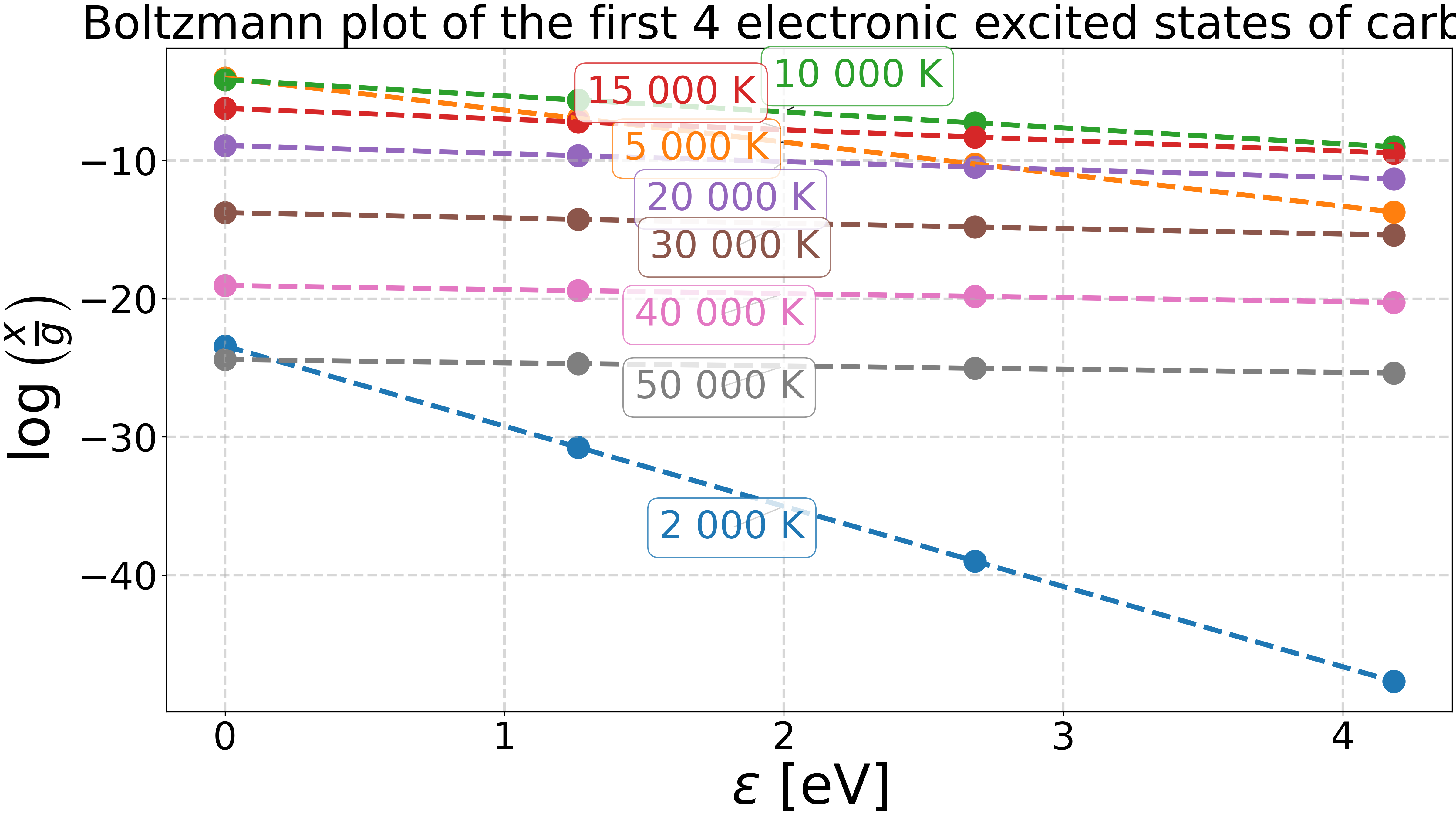
—

Boltzmann plot of the first electronic excited states of carbon.

The equilibrium is computed via Cantera at a given temperature and pressure.

From Boltzmann equation, we have:

\[n_\text{u} = n_0 \frac{g_\text{u} \exp\left(-\frac{E_\text{u}}{k_\text{B} T}\right)}{Z(T)}\]

Dividing by the total density, and rearranging terms, we obtain:

\[\log\left(\frac{x_\text{u}}{g_\text{u}}\right) = \log\left(\frac{x_\text{0}}{Z(T)}\right) -\frac{E_\text{u}}{k_\text{B} T}\]

Tags: kinetics equilibrium reverse reaction CH4 C2H2 Janev

# This is an option for the online documentation, so that each image is displayed separately.
# sphinx_gallery_multi_image = "single"

Import the required libraries.

import cantera as ct
import matplotlib.pyplot as plt
import numpy as np
from adjustText import adjust_text

import rizer.misc.units as u
from rizer.kin.extensible_rate import *  # noqa: F403
from rizer.misc.plt_utils import set_mpl_style
from rizer.misc.utils import get_path_to_data

set_mpl_style(nb_columns=1)

Define mechanisms and parameters.

mechanism = get_path_to_data(
    "mechanisms",
    "Goutier2025",
    "CH4_to_C2H2.yaml",
)

gas = ct.Solution(mechanism, name="gas_with_electronic_excited_states")
assert "C(1D)" in gas.species_names


# Temperatures in Kelvin.
temperatures = np.array([2000, 5000, 10000, 15000, 20000, 30000, 40000, 50000])
# Pressure in Pascals.
P = ct.one_atm
# Initial mole fraction (here, we start with pure methane).
X_0 = "CH4:1"

# Energy and degenaracy of the first electronic excited states of carbon.
# cf. https://physics.nist.gov/cgi-bin/ASD/energy1.pl?de=0&spectrum=C+I&units=1&format=0&output=0&page_size=15&multiplet_ordered=0&conf_out=on&term_out=on&level_out=on&unc_out=1&j_out=on&g_out=on&lande_out=on&perc_out=on&biblio=on&temp=&submit=Retrieve+Data
energies_eV = np.array([0.0, 1.2637284, 2.6840136, 4.1826219])
gs = np.array([9, 5, 1, 5])

Plot the Boltzmann plot.

fig, ax = plt.subplots()

texts = []
for T in temperatures:
    # Equilibrate the mixture.
    gas.TPX = T, P, X_0
    gas.equilibrate("TP")
    # Get the mole fraction.
    X = gas["C", "C(1D)", "C(1S)", "C(5So)"].X

    # Plot log(x/g) vs energy
    ax.scatter(energies_eV, np.log(X / gs), marker="o", s=300)

    # Fit data to `y=b-a*x`
    coefs = np.polynomial.polynomial.polyfit(x=energies_eV, y=np.log(X / gs), deg=1)
    ax.plot(
        energies_eV,
        np.polynomial.polynomial.polyval(energies_eV, coefs),
        ls="--",
        lw=4,
    )

    # Get back the temperature.
    # y = b - a*x
    a_per_eV = -coefs[1]  # eV^(-1)
    a_per_J = a_per_eV / (u.eV_to_J)  # J^(-1)
    # a = 1/(k_B * T)
    T_fit = 1 / (a_per_J * u.k_b)  # K
    print(f"Temperature from fit: {T_fit:.2e} K")

    # Annotate at 2 eV.
    texts.append(
        ax.text(
            x=2,
            y=float(np.polynomial.polynomial.polyval(2, coefs)),
            s=f"{int(T_fit):,} K".replace(",", " "),
            color=ax.lines[-1].get_color(),
            horizontalalignment="center",
            verticalalignment="center",
            bbox=dict(
                facecolor="white",
                alpha=0.8,
                edgecolor=ax.lines[-1].get_color(),
                boxstyle="round",
            ),
        )
    )

ax.set_xlabel(r"$\varepsilon$ [eV]")
ax.set_ylabel(r"$\log\left(\frac{x}{g}\right)$")
ax.set_title("Boltzmann plot of the first 4 electronic excited states of carbon.")
adjust_text(texts, arrowprops=dict(arrowstyle="->", color="k"))
plt.show()

Temperature from fit: 2.00e+03 K
Temperature from fit: 5.00e+03 K
Temperature from fit: 1.00e+04 K
Temperature from fit: 1.50e+04 K
Temperature from fit: 2.00e+04 K
Temperature from fit: 3.00e+04 K
Temperature from fit: 4.00e+04 K
Temperature from fit: 5.00e+04 K