—

Plot CH₄ average and elastic momentum transfer cross sections.

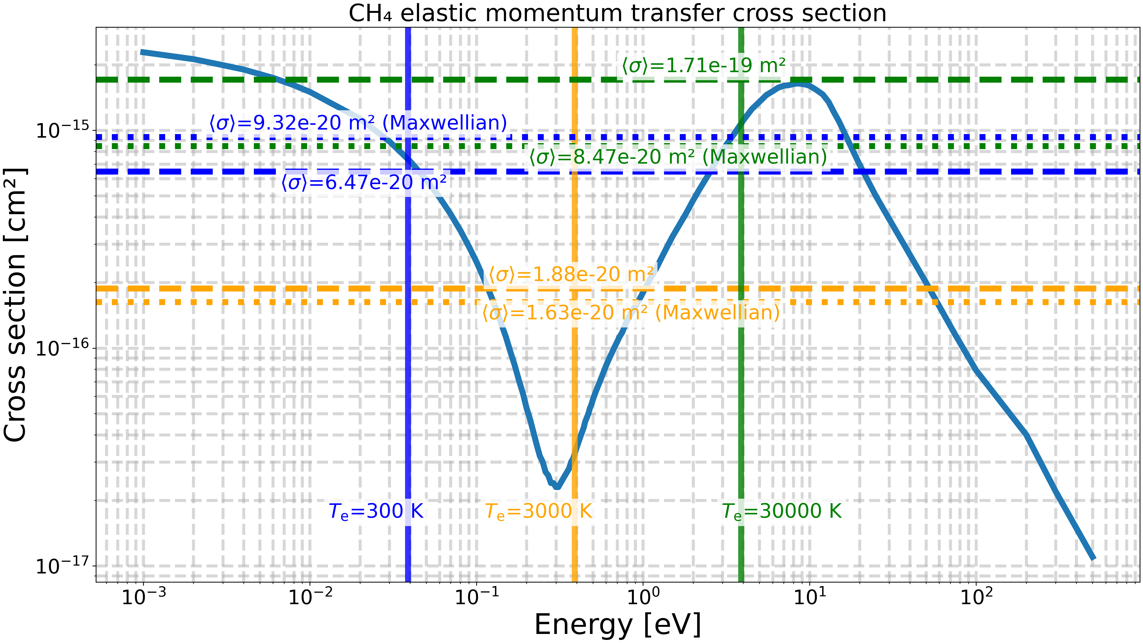
The elastic cross section of methane (CH₄) is plotted as a function of the electron energy. Data is taken from the Song Bouwman database, which is available on the LXCat website. This cross section corresponds to the collision process e- + CH₄ -> e- + CH₄, which is an elastic collision where the electron is scattered by the methane molecule without any energy loss.

Using [Mitchner1973] notation, this corresponds to the elastic momentum transfer cross section \(Q_{12}^{(1)}(\varepsilon)\).

From it, an average momentum transfer cross section is computed (see Eq. II-6.30 in [Mitchner1973]), obtained assuming a Maxwellian distribution of electron energies at different electron temperatures. (It is also assumed that methane follows a Maxwellian distribution).

An average momentum transfer cross section is also computed using (not defined in [Mitchner1973]):

\[\bar{Q}_{12} = \int_0^{\infty} \tilde{Q_{12}}^{(1)}(\varepsilon) f_T(\varepsilon) d\varepsilon\]

where:

• \(\bar{Q}_{12}\) is the average momentum transfer cross section, in m^2,

• \(\tilde{Q_{12}}^{(1)}(\varepsilon)\) is the (energy) momentum transfer cross section, in m^2,

• \(f_T(\varepsilon)\) is the Maxwellian distribution function, in J^-1,

• \(\varepsilon\) is the kinetic energy of the electron, in J.

Notes

• \(Q_{12}^{(e)}(g)\) is the (velocity) elastic cross section, in m^2, (depending on the relative velocity \(g\)), defined in equation (II 3.5) of [Mitchner1973].

• \(Q_{12}^{(1)}(g)\) is the (velocity) momentum transfer cross section, in m^2, (depending on the relative velocity \(g\)), defined in equation (II 3.7) of [Mitchner1973].

Tags: cross sections momentum transfer TabulatedSpeciesCrossSection HardSphereCrossSection LXCat

Import the required libraries.

import matplotlib.pyplot as plt
import numpy as np
from adjustText import adjust_text

import rizer.misc.units as u
from rizer.io.lxcat import Collision, LXCat
from rizer.misc.plt_utils import set_mpl_style
from rizer.misc.utils import get_path_to_data
from rizer.plasma.momentum_transfer_cross_sections import TabulatedSpeciesCrossSection

set_mpl_style()

Load the cross section data.

# Load the cross section data from the Song Bouwman database.
lx = LXCat(verbose=False)
lx.read(file=get_path_to_data("kin", "cross_section", "CH4", "SongBouwman.txt"))

# Get the elastic momentum transfer cross section data of methane (e- + CH₄ -> e- + CH₄).
df: Collision = lx.species["CH4"].collisions["CH4"]

# Create a TabulatedSpeciesCrossSection model with the cross section data.
cross_section_m2 = df.cross_section_cm2 * 1e-4  # Convert cm² to m².
energy_J = df.energy_eV * u.eV_to_J  # Convert eV to J.
model = TabulatedSpeciesCrossSection(
    cross_section_m2=cross_section_m2, energy_J=energy_J
)
# Compute the mean cross section for some electron temperature.
electron_temperatures = [300, 3000, 30000]  # K
colors = ["blue", "orange", "green"]
average_cross_sections: list[float] = []
for T_e in electron_temperatures:
    mean_cross_section = model.get_mean_cross_section(T_e=T_e)
    average_cross_sections.append(mean_cross_section)
    print(f"Mean cross section at T_e={T_e} K: {mean_cross_section:.2e} m²")

# Compare with the mean cross section computed from the Maxwellian distribution.
average_cross_sections_maxwellian: list[float] = []
for T_e in electron_temperatures:
    mean_cross_section_maxwellian = model.get_mean_cross_section_from_maxwellian(
        T_e=T_e
    )
    average_cross_sections_maxwellian.append(mean_cross_section_maxwellian)
    print(
        f"Mean cross section (Maxwellian) at T_e={T_e} K: {mean_cross_section_maxwellian:.2e} m²"
    )

Mean cross section at T_e=300 K: 6.47e-20 m²
Mean cross section at T_e=3000 K: 1.88e-20 m²
Mean cross section at T_e=30000 K: 1.71e-19 m²
Mean cross section (Maxwellian) at T_e=300 K: 9.32e-20 m²
Mean cross section (Maxwellian) at T_e=3000 K: 1.63e-20 m²
Mean cross section (Maxwellian) at T_e=30000 K: 8.47e-20 m²

Plot the cross sections.

fig, ax = plt.subplots()

# Plot the original cross section data.
ax.plot(df.energy_eV, df.cross_section_cm2)

# Plot the mean cross sections as horizontal lines and the corresponding energies as vertical lines.
texts = []
for T_e, mean_cs, color in zip(electron_temperatures, average_cross_sections, colors):
    ax.axhline(
        mean_cs * 1e4,
        # label=f"T_e={T_e} K = {1.5 * T_e * u.K_to_eV:.1e} eV",
        linestyle="--",
        color=color,
    )
    texts.append(
        ax.text(
            1.5 * T_e * u.K_to_eV,
            mean_cs * 1e4,
            rf"$\langle\sigma\rangle$={mean_cs:.2e} m²",
            color=color,
            va="center",
            ha="center",
            bbox=dict(facecolor="white", alpha=0.8, edgecolor="none"),
        )
    )

    ax.axvline(
        1.5 * T_e * u.K_to_eV,
        linestyle="-",
        color=color,
        alpha=0.8,
    )
    texts.append(
        ax.text(
            1.5 * T_e * u.K_to_eV,
            2e-17,
            rf"$T_\mathrm{{e}}$={T_e} K",
            color=color,
            va="center",
            ha="center",
            bbox=dict(facecolor="white", alpha=0.8, edgecolor="none"),
        )
    )
for T_e, mean_cs_maxwellian, color in zip(
    electron_temperatures, average_cross_sections_maxwellian, colors
):
    ax.axhline(
        mean_cs_maxwellian * 1e4,
        label=f"T_e={T_e} K = {1.5 * T_e * u.K_to_eV:.1e} eV (Maxwellian)",
        linestyle=":",
        color=color,
    )
    texts.append(
        ax.text(
            1.5 * T_e * u.K_to_eV,
            mean_cs_maxwellian * 1e4,
            rf"$\langle\sigma\rangle$={mean_cs_maxwellian:.2e} m² (Maxwellian)",
            color=color,
            va="center",
            ha="center",
            bbox=dict(facecolor="white", alpha=0.8, edgecolor="none"),
        )
    )

ax.set_xlabel("Energy [eV]")
ax.set_ylabel("Cross section [cm²]")
ax.set_title("CH₄ elastic momentum transfer cross section")
ax.set_xscale("log")
ax.set_yscale("log")
adjust_text(texts)
plt.show()

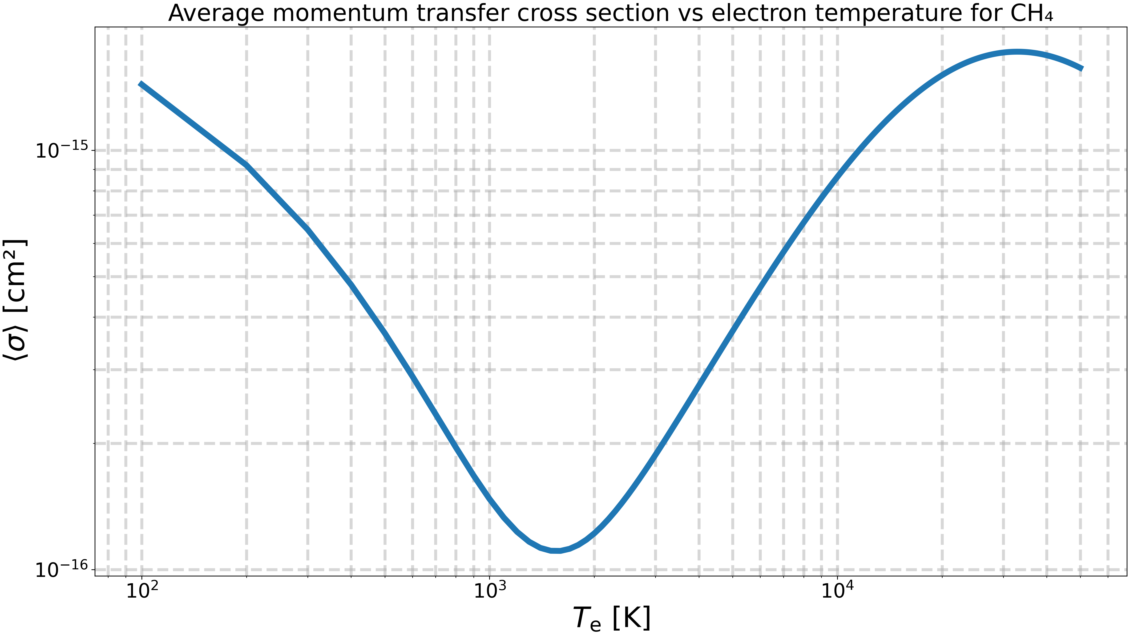
Compute and plot the average momentum transfer cross section as a function of the electron temperature.

T_e_s = np.arange(100, 50000, 100, dtype=float)  # K
average_cross_sections_Te: list[float] = []

for T_e in T_e_s:
    mean_cross_section = model.get_mean_cross_section(T_e=T_e)
    average_cross_sections_Te.append(mean_cross_section * 1e4)  # Convert m² to cm².

fig, ax = plt.subplots()
ax.plot(T_e_s, average_cross_sections_Te)
ax.set_xlabel(r"$T_\mathrm{e}$ [K]")
ax.set_ylabel(r"$\langle\sigma\rangle$ [cm²]")
ax.set_title("Average momentum transfer cross section vs electron temperature for CH₄")
ax.set_xscale("log")
ax.set_yscale("log")
plt.show()

# One effect of averaging the cross section is the diminution of the amplitude of the resonances,
# which are smoothed out by the averaging process.