—
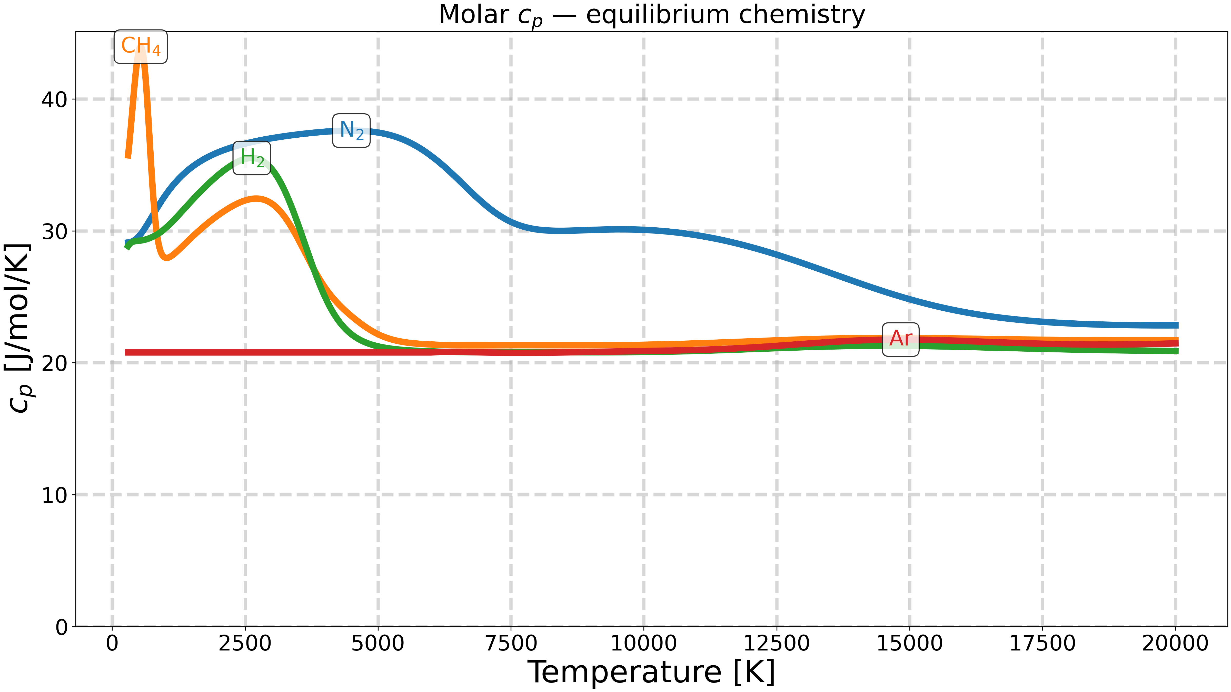
Plot molar heat capacity of N₂, CH₄, H₂ and Ar vs. temperature.#
This example demonstrates how to compute and plot the molar heat capacity at constant pressure (\(c_p\)) of N₂, CH₄, H₂ and Ar as a function of temperature, from 300 to 20 000 K.
At each temperature the mixture is brought to chemical equilibrium at
constant T and P starting from one mole of the pure species. The
resulting \(c_p\) is Cantera’s frozen-composition heat capacity
cp_mole evaluated at the equilibrium composition,
expressed in J/mol/K.
The thermo data (NASA 9-polynomial) come from the GRC database.
Note
The temperature range of CH₄ is limited to 6 000 K by its NASA 9 polynomial fit, while N₂, H₂ and Ar are available up to 20 000 K.
See also
Plot specific heat vs. temperature for different species and thermo data. – plots the single-species \(c_p\) across several thermo databases for C/H species.
Plot thermodynamic properties of H₂ vs. temperatures. – plots the mass heat capacity of H₂ in LTE conditions.
Import the required libraries.#
import cantera as ct
import matplotlib.pyplot as plt
import numpy as np

from rizer.misc.plt_utils import (
    get_species_color,
    get_species_in_latex,
    get_text,
    set_mpl_style,
)
from rizer.misc.utils import get_path_to_data

set_mpl_style(nb_columns=1)
Load species from the GRC NASA 9 database.#
The file grc_nasa9_all.yaml contains NASA 9-polynomial thermo data for a
wide range of atomic and molecular species, covering temperatures up to
20 000 K for most species.
path_to_thermo = get_path_to_data("mechanisms/thermo", "grc_nasa9_all.yaml")
all_species: list[ct.Species] = ct.Species.list_from_file(str(path_to_thermo))
species_by_name: dict[str, ct.Species] = {s.name: s for s in all_species}
Compute the equilibrium molar cp for each species.#
For each species a single-species ideal-gas is created and equilibrated at
each temperature using equilibrate().
cp_mole gives the frozen-composition molar
heat capacity [J/kmol/K] of the mixture. Dividing by 1 000 converts to
J/mol/K.
T_min = 300.0  # K
T_max = 20_000.0  # K
n_points = 1000

species_names = ["N2", "CH4", "H2", "Ar"]
Equilibrium chemistry.#
The gas is equilibrated at each temperature before reading
cp_mole.
# To compute the equilibrium composition, we need to create a gas object that
# contains all the species.  We load all the species from the GRC NASA 9
# database, then filter out any species that contain elements other than N, C, H
# and Ar to accelerate the computation.
all_species = ct.Species.list_from_file(str(path_to_thermo))
all_species = [
    s for s in all_species if set(s.composition).issubset({"N", "C", "H", "Ar", "E"})
]

gas = ct.Solution(thermo="ideal-gas", kinetics="gas", species=all_species)
fig, ax = plt.subplots()

for name in species_names:
    temperatures = np.linspace(T_min, T_max, n_points)

    states = ct.SolutionArray(gas, shape=temperatures.shape)
    states.TPX = temperatures, ct.one_atm, f"{name}:1"
    states.equilibrate("TP")

    cp_molar = states.cp_mole / 1e3  # J/kmol/K → J/mol/K

    color = get_species_color(name)
    ax.plot(temperatures, cp_molar, color=color)
    get_text(
        float(temperatures[np.argmax(cp_molar)]),
        float(np.max(cp_molar)),
        get_species_in_latex(name),
        ax=ax,
        color=color,
    )

ax.set_xlabel("Temperature [K]")
ax.set_ylabel(r"$c_p$ [J/mol/K]")
ax.set_title(r"Molar $c_p$ — equilibrium chemistry")
ax.set_ylim(bottom=0)

plt.show()
/home/runner/micromamba/envs/DEVELOP/lib/python3.14/site-packages/cantera/composite.py:866: UserWarning: ChemEquil::equilibrate: Temperature (5013.01301301301 K) outside valid range of 300 K to 5000 K
  self._phase.equilibrate(*args, **kwargs)
/home/runner/micromamba/envs/DEVELOP/lib/python3.14/site-packages/cantera/composite.py:866: UserWarning: ChemEquil::equilibrate: Temperature (5032.732732732737 K) outside valid range of 300 K to 5000 K
  self._phase.equilibrate(*args, **kwargs)
/home/runner/micromamba/envs/DEVELOP/lib/python3.14/site-packages/cantera/composite.py:866: UserWarning: ChemEquil::equilibrate: Temperature (5052.45245245245 K) outside valid range of 300 K to 5000 K
  self._phase.equilibrate(*args, **kwargs)
/home/runner/micromamba/envs/DEVELOP/lib/python3.14/site-packages/cantera/composite.py:866: UserWarning: ChemEquil::equilibrate: Temperature (5072.172172172169 K) outside valid range of 300 K to 5000 K
  self._phase.equilibrate(*args, **kwargs)
/home/runner/micromamba/envs/DEVELOP/lib/python3.14/site-packages/cantera/composite.py:866: UserWarning: ChemEquil::equilibrate: Temperature (5091.891891891893 K) outside valid range of 300 K to 5000 K
  self._phase.equilibrate(*args, **kwargs)
/home/runner/micromamba/envs/DEVELOP/lib/python3.14/site-packages/cantera/composite.py:866: UserWarning: ChemEquil::equilibrate: Temperature (5111.611611611615 K) outside valid range of 300 K to 5000 K
  self._phase.equilibrate(*args, **kwargs)
/home/runner/micromamba/envs/DEVELOP/lib/python3.14/site-packages/cantera/composite.py:866: UserWarning: ChemEquil::equilibrate: Temperature (5131.33133133133 K) outside valid range of 300 K to 5000 K
  self._phase.equilibrate(*args, **kwargs)
/home/runner/micromamba/envs/DEVELOP/lib/python3.14/site-packages/cantera/composite.py:866: UserWarning: ChemEquil::equilibrate: Temperature (5151.051051051056 K) outside valid range of 300 K to 5000 K
  self._phase.equilibrate(*args, **kwargs)
/home/runner/micromamba/envs/DEVELOP/lib/python3.14/site-packages/cantera/composite.py:866: UserWarning: ChemEquil::equilibrate: Temperature (5170.7707707707705 K) outside valid range of 300 K to 5000 K
  self._phase.equilibrate(*args, **kwargs)
/home/runner/micromamba/envs/DEVELOP/lib/python3.14/site-packages/cantera/composite.py:866: UserWarning: ChemEquil::equilibrate: Temperature (5190.490490490494 K) outside valid range of 300 K to 5000 K
  self._phase.equilibrate(*args, **kwargs)
/home/runner/micromamba/envs/DEVELOP/lib/python3.14/site-packages/cantera/composite.py:866: UserWarning: ChemEquil::equilibrate: Temperature (5210.21021021021 K) outside valid range of 300 K to 5000 K
  self._phase.equilibrate(*args, **kwargs)
/home/runner/micromamba/envs/DEVELOP/lib/python3.14/site-packages/cantera/composite.py:866: UserWarning: ChemEquil::equilibrate: Temperature (5229.929929929929 K) outside valid range of 300 K to 5000 K
  self._phase.equilibrate(*args, **kwargs)
/home/runner/micromamba/envs/DEVELOP/lib/python3.14/site-packages/cantera/composite.py:866: UserWarning: ChemEquil::equilibrate: Temperature (5249.649649649651 K) outside valid range of 300 K to 5000 K
  self._phase.equilibrate(*args, **kwargs)
/home/runner/micromamba/envs/DEVELOP/lib/python3.14/site-packages/cantera/composite.py:866: UserWarning: ChemEquil::equilibrate: Temperature (5269.369369369366 K) outside valid range of 300 K to 5000 K
  self._phase.equilibrate(*args, **kwargs)
/home/runner/micromamba/envs/DEVELOP/lib/python3.14/site-packages/cantera/composite.py:866: UserWarning: ChemEquil::equilibrate: Temperature (5289.089089089088 K) outside valid range of 300 K to 5000 K
  self._phase.equilibrate(*args, **kwargs)
/home/runner/micromamba/envs/DEVELOP/lib/python3.14/site-packages/cantera/composite.py:866: UserWarning: ChemEquil::equilibrate: Temperature (5308.808808808807 K) outside valid range of 300 K to 5000 K
  self._phase.equilibrate(*args, **kwargs)
/home/runner/micromamba/envs/DEVELOP/lib/python3.14/site-packages/cantera/composite.py:866: UserWarning: ChemEquil::equilibrate: Temperature (5328.528528528529 K) outside valid range of 300 K to 5000 K
  self._phase.equilibrate(*args, **kwargs)
/home/runner/micromamba/envs/DEVELOP/lib/python3.14/site-packages/cantera/composite.py:866: UserWarning: ChemEquil::equilibrate: Temperature (5348.248248248249 K) outside valid range of 300 K to 5000 K
  self._phase.equilibrate(*args, **kwargs)
/home/runner/micromamba/envs/DEVELOP/lib/python3.14/site-packages/cantera/composite.py:866: UserWarning: ChemEquil::equilibrate: Temperature (5367.967967967966 K) outside valid range of 300 K to 5000 K
  self._phase.equilibrate(*args, **kwargs)
/home/runner/micromamba/envs/DEVELOP/lib/python3.14/site-packages/cantera/composite.py:866: UserWarning: ChemEquil::equilibrate: Temperature (5387.687687687684 K) outside valid range of 300 K to 5000 K
  self._phase.equilibrate(*args, **kwargs)
/home/runner/micromamba/envs/DEVELOP/lib/python3.14/site-packages/cantera/composite.py:866: UserWarning: ChemEquil::equilibrate: Temperature (5407.407407407405 K) outside valid range of 300 K to 5000 K
  self._phase.equilibrate(*args, **kwargs)
/home/runner/micromamba/envs/DEVELOP/lib/python3.14/site-packages/cantera/composite.py:866: UserWarning: ChemEquil::equilibrate: Temperature (5427.127127127128 K) outside valid range of 300 K to 5000 K
  self._phase.equilibrate(*args, **kwargs)
/home/runner/micromamba/envs/DEVELOP/lib/python3.14/site-packages/cantera/composite.py:866: UserWarning: ChemEquil::equilibrate: Temperature (5446.84684684685 K) outside valid range of 300 K to 5000 K
  self._phase.equilibrate(*args, **kwargs)
/home/runner/micromamba/envs/DEVELOP/lib/python3.14/site-packages/cantera/composite.py:866: UserWarning: ChemEquil::equilibrate: Temperature (5466.566566566563 K) outside valid range of 300 K to 5000 K
  self._phase.equilibrate(*args, **kwargs)
/home/runner/micromamba/envs/DEVELOP/lib/python3.14/site-packages/cantera/composite.py:866: UserWarning: ChemEquil::equilibrate: Temperature (5486.286286286291 K) outside valid range of 300 K to 5000 K
  self._phase.equilibrate(*args, **kwargs)
/home/runner/micromamba/envs/DEVELOP/lib/python3.14/site-packages/cantera/composite.py:866: UserWarning: ChemEquil::equilibrate: Temperature (5506.006006006003 K) outside valid range of 300 K to 5000 K
  self._phase.equilibrate(*args, **kwargs)
/home/runner/micromamba/envs/DEVELOP/lib/python3.14/site-packages/cantera/composite.py:866: UserWarning: ChemEquil::equilibrate: Temperature (5525.725725725725 K) outside valid range of 300 K to 5000 K
  self._phase.equilibrate(*args, **kwargs)
/home/runner/micromamba/envs/DEVELOP/lib/python3.14/site-packages/cantera/composite.py:866: UserWarning: ChemEquil::equilibrate: Temperature (5545.445445445445 K) outside valid range of 300 K to 5000 K
  self._phase.equilibrate(*args, **kwargs)
/home/runner/micromamba/envs/DEVELOP/lib/python3.14/site-packages/cantera/composite.py:866: UserWarning: ChemEquil::equilibrate: Temperature (5565.1651651651655 K) outside valid range of 300 K to 5000 K
  self._phase.equilibrate(*args, **kwargs)
/home/runner/micromamba/envs/DEVELOP/lib/python3.14/site-packages/cantera/composite.py:866: UserWarning: ChemEquil::equilibrate: Temperature (5584.884884884887 K) outside valid range of 300 K to 5000 K
  self._phase.equilibrate(*args, **kwargs)
/home/runner/micromamba/envs/DEVELOP/lib/python3.14/site-packages/cantera/composite.py:866: UserWarning: ChemEquil::equilibrate: Temperature (5604.604604604605 K) outside valid range of 300 K to 5000 K
  self._phase.equilibrate(*args, **kwargs)
/home/runner/micromamba/envs/DEVELOP/lib/python3.14/site-packages/cantera/composite.py:866: UserWarning: ChemEquil::equilibrate: Temperature (5624.324324324322 K) outside valid range of 300 K to 5000 K
  self._phase.equilibrate(*args, **kwargs)
/home/runner/micromamba/envs/DEVELOP/lib/python3.14/site-packages/cantera/composite.py:866: UserWarning: ChemEquil::equilibrate: Temperature (5644.044044044044 K) outside valid range of 300 K to 5000 K
  self._phase.equilibrate(*args, **kwargs)
/home/runner/micromamba/envs/DEVELOP/lib/python3.14/site-packages/cantera/composite.py:866: UserWarning: ChemEquil::equilibrate: Temperature (5663.763763763762 K) outside valid range of 300 K to 5000 K
  self._phase.equilibrate(*args, **kwargs)
/home/runner/micromamba/envs/DEVELOP/lib/python3.14/site-packages/cantera/composite.py:866: UserWarning: ChemEquil::equilibrate: Temperature (5683.483483483483 K) outside valid range of 300 K to 5000 K
  self._phase.equilibrate(*args, **kwargs)
/home/runner/micromamba/envs/DEVELOP/lib/python3.14/site-packages/cantera/composite.py:866: UserWarning: ChemEquil::equilibrate: Temperature (5703.2032032032 K) outside valid range of 300 K to 5000 K
  self._phase.equilibrate(*args, **kwargs)
/home/runner/micromamba/envs/DEVELOP/lib/python3.14/site-packages/cantera/composite.py:866: UserWarning: ChemEquil::equilibrate: Temperature (5722.92292292292 K) outside valid range of 300 K to 5000 K
  self._phase.equilibrate(*args, **kwargs)
/home/runner/micromamba/envs/DEVELOP/lib/python3.14/site-packages/cantera/composite.py:866: UserWarning: ChemEquil::equilibrate: Temperature (5742.642642642644 K) outside valid range of 300 K to 5000 K
  self._phase.equilibrate(*args, **kwargs)
/home/runner/micromamba/envs/DEVELOP/lib/python3.14/site-packages/cantera/composite.py:866: UserWarning: ChemEquil::equilibrate: Temperature (5762.362362362365 K) outside valid range of 300 K to 5000 K
  self._phase.equilibrate(*args, **kwargs)
/home/runner/micromamba/envs/DEVELOP/lib/python3.14/site-packages/cantera/composite.py:866: UserWarning: ChemEquil::equilibrate: Temperature (5782.082082082079 K) outside valid range of 300 K to 5000 K
  self._phase.equilibrate(*args, **kwargs)
/home/runner/micromamba/envs/DEVELOP/lib/python3.14/site-packages/cantera/composite.py:866: UserWarning: ChemEquil::equilibrate: Temperature (5801.801801801798 K) outside valid range of 300 K to 5000 K
  self._phase.equilibrate(*args, **kwargs)
/home/runner/micromamba/envs/DEVELOP/lib/python3.14/site-packages/cantera/composite.py:866: UserWarning: ChemEquil::equilibrate: Temperature (5821.521521521517 K) outside valid range of 300 K to 5000 K
  self._phase.equilibrate(*args, **kwargs)
/home/runner/micromamba/envs/DEVELOP/lib/python3.14/site-packages/cantera/composite.py:866: UserWarning: ChemEquil::equilibrate: Temperature (5841.241241241241 K) outside valid range of 300 K to 5000 K
  self._phase.equilibrate(*args, **kwargs)
/home/runner/micromamba/envs/DEVELOP/lib/python3.14/site-packages/cantera/composite.py:866: UserWarning: ChemEquil::equilibrate: Temperature (5860.9609609609615 K) outside valid range of 300 K to 5000 K
  self._phase.equilibrate(*args, **kwargs)
/home/runner/micromamba/envs/DEVELOP/lib/python3.14/site-packages/cantera/composite.py:866: UserWarning: ChemEquil::equilibrate: Temperature (5880.6806806806835 K) outside valid range of 300 K to 5000 K
  self._phase.equilibrate(*args, **kwargs)
/home/runner/micromamba/envs/DEVELOP/lib/python3.14/site-packages/cantera/composite.py:866: UserWarning: ChemEquil::equilibrate: Temperature (5900.400400400398 K) outside valid range of 300 K to 5000 K
  self._phase.equilibrate(*args, **kwargs)
/home/runner/micromamba/envs/DEVELOP/lib/python3.14/site-packages/cantera/composite.py:866: UserWarning: ChemEquil::equilibrate: Temperature (5920.120120120124 K) outside valid range of 300 K to 5000 K
  self._phase.equilibrate(*args, **kwargs)
/home/runner/micromamba/envs/DEVELOP/lib/python3.14/site-packages/cantera/composite.py:866: UserWarning: ChemEquil::equilibrate: Temperature (5939.839839839834 K) outside valid range of 300 K to 5000 K
  self._phase.equilibrate(*args, **kwargs)
/home/runner/micromamba/envs/DEVELOP/lib/python3.14/site-packages/cantera/composite.py:866: UserWarning: ChemEquil::equilibrate: Temperature (5959.559559559558 K) outside valid range of 300 K to 5000 K
  self._phase.equilibrate(*args, **kwargs)
/home/runner/micromamba/envs/DEVELOP/lib/python3.14/site-packages/cantera/composite.py:866: UserWarning: ChemEquil::equilibrate: Temperature (5979.279279279273 K) outside valid range of 300 K to 5000 K
  self._phase.equilibrate(*args, **kwargs)
/home/runner/micromamba/envs/DEVELOP/lib/python3.14/site-packages/cantera/composite.py:866: UserWarning: ChemEquil::equilibrate: Temperature (5998.998998999004 K) outside valid range of 300 K to 5000 K
  self._phase.equilibrate(*args, **kwargs)
/home/runner/micromamba/envs/DEVELOP/lib/python3.14/site-packages/cantera/composite.py:866: UserWarning: ChemEquil::equilibrate: Temperature (6018.71871871872 K) outside valid range of 300 K to 5000 K
  self._phase.equilibrate(*args, **kwargs)
/home/runner/micromamba/envs/DEVELOP/lib/python3.14/site-packages/cantera/composite.py:866: UserWarning: ChemEquil::equilibrate: Temperature (6038.438438438434 K) outside valid range of 300 K to 5000 K
  self._phase.equilibrate(*args, **kwargs)
/home/runner/micromamba/envs/DEVELOP/lib/python3.14/site-packages/cantera/composite.py:866: UserWarning: ChemEquil::equilibrate: Temperature (6058.158158158161 K) outside valid range of 300 K to 5000 K
  self._phase.equilibrate(*args, **kwargs)
/home/runner/micromamba/envs/DEVELOP/lib/python3.14/site-packages/cantera/composite.py:866: UserWarning: ChemEquil::equilibrate: Temperature (6077.877877877879 K) outside valid range of 300 K to 5000 K
  self._phase.equilibrate(*args, **kwargs)
/home/runner/micromamba/envs/DEVELOP/lib/python3.14/site-packages/cantera/composite.py:866: UserWarning: ChemEquil::equilibrate: Temperature (6097.597597597598 K) outside valid range of 300 K to 5000 K
  self._phase.equilibrate(*args, **kwargs)
/home/runner/micromamba/envs/DEVELOP/lib/python3.14/site-packages/cantera/composite.py:866: UserWarning: ChemEquil::equilibrate: Temperature (6117.317317317313 K) outside valid range of 300 K to 5000 K
  self._phase.equilibrate(*args, **kwargs)
/home/runner/micromamba/envs/DEVELOP/lib/python3.14/site-packages/cantera/composite.py:866: UserWarning: ChemEquil::equilibrate: Temperature (6137.037037037037 K) outside valid range of 300 K to 5000 K
  self._phase.equilibrate(*args, **kwargs)
/home/runner/micromamba/envs/DEVELOP/lib/python3.14/site-packages/cantera/composite.py:866: UserWarning: ChemEquil::equilibrate: Temperature (6156.756756756762 K) outside valid range of 300 K to 5000 K
  self._phase.equilibrate(*args, **kwargs)
/home/runner/micromamba/envs/DEVELOP/lib/python3.14/site-packages/cantera/composite.py:866: UserWarning: ChemEquil::equilibrate: Temperature (6176.476476476479 K) outside valid range of 300 K to 5000 K
  self._phase.equilibrate(*args, **kwargs)
/home/runner/micromamba/envs/DEVELOP/lib/python3.14/site-packages/cantera/composite.py:866: UserWarning: ChemEquil::equilibrate: Temperature (6196.1961961962 K) outside valid range of 300 K to 5000 K
  self._phase.equilibrate(*args, **kwargs)
/home/runner/micromamba/envs/DEVELOP/lib/python3.14/site-packages/cantera/composite.py:866: UserWarning: ChemEquil::equilibrate: Temperature (6215.915915915921 K) outside valid range of 300 K to 5000 K
  self._phase.equilibrate(*args, **kwargs)
/home/runner/micromamba/envs/DEVELOP/lib/python3.14/site-packages/cantera/composite.py:866: UserWarning: ChemEquil::equilibrate: Temperature (6235.635635635635 K) outside valid range of 300 K to 5000 K
  self._phase.equilibrate(*args, **kwargs)
/home/runner/micromamba/envs/DEVELOP/lib/python3.14/site-packages/cantera/composite.py:866: UserWarning: ChemEquil::equilibrate: Temperature (6255.3553553553575 K) outside valid range of 300 K to 5000 K
  self._phase.equilibrate(*args, **kwargs)
/home/runner/micromamba/envs/DEVELOP/lib/python3.14/site-packages/cantera/composite.py:866: UserWarning: ChemEquil::equilibrate: Temperature (6275.075075075079 K) outside valid range of 300 K to 5000 K
  self._phase.equilibrate(*args, **kwargs)
/home/runner/micromamba/envs/DEVELOP/lib/python3.14/site-packages/cantera/composite.py:866: UserWarning: ChemEquil::equilibrate: Temperature (6294.794794794793 K) outside valid range of 300 K to 5000 K
  self._phase.equilibrate(*args, **kwargs)
/home/runner/micromamba/envs/DEVELOP/lib/python3.14/site-packages/cantera/composite.py:866: UserWarning: ChemEquil::equilibrate: Temperature (6314.51451451451 K) outside valid range of 300 K to 5000 K
  self._phase.equilibrate(*args, **kwargs)
/home/runner/micromamba/envs/DEVELOP/lib/python3.14/site-packages/cantera/composite.py:866: UserWarning: ChemEquil::equilibrate: Temperature (6334.234234234237 K) outside valid range of 300 K to 5000 K
  self._phase.equilibrate(*args, **kwargs)
/home/runner/micromamba/envs/DEVELOP/lib/python3.14/site-packages/cantera/composite.py:866: UserWarning: ChemEquil::equilibrate: Temperature (6353.953953953951 K) outside valid range of 300 K to 5000 K
  self._phase.equilibrate(*args, **kwargs)
/home/runner/micromamba/envs/DEVELOP/lib/python3.14/site-packages/cantera/composite.py:866: UserWarning: ChemEquil::equilibrate: Temperature (6373.673673673679 K) outside valid range of 300 K to 5000 K
  self._phase.equilibrate(*args, **kwargs)
/home/runner/micromamba/envs/DEVELOP/lib/python3.14/site-packages/cantera/composite.py:866: UserWarning: ChemEquil::equilibrate: Temperature (6393.393393393396 K) outside valid range of 300 K to 5000 K
  self._phase.equilibrate(*args, **kwargs)
/home/runner/micromamba/envs/DEVELOP/lib/python3.14/site-packages/cantera/composite.py:866: UserWarning: ChemEquil::equilibrate: Temperature (6413.113113113115 K) outside valid range of 300 K to 5000 K
  self._phase.equilibrate(*args, **kwargs)
/home/runner/micromamba/envs/DEVELOP/lib/python3.14/site-packages/cantera/composite.py:866: UserWarning: ChemEquil::equilibrate: Temperature (6432.832832832827 K) outside valid range of 300 K to 5000 K
  self._phase.equilibrate(*args, **kwargs)
/home/runner/micromamba/envs/DEVELOP/lib/python3.14/site-packages/cantera/composite.py:866: UserWarning: ChemEquil::equilibrate: Temperature (6452.552552552553 K) outside valid range of 300 K to 5000 K
  self._phase.equilibrate(*args, **kwargs)
/home/runner/micromamba/envs/DEVELOP/lib/python3.14/site-packages/cantera/composite.py:866: UserWarning: ChemEquil::equilibrate: Temperature (6472.272272272268 K) outside valid range of 300 K to 5000 K
  self._phase.equilibrate(*args, **kwargs)
/home/runner/micromamba/envs/DEVELOP/lib/python3.14/site-packages/cantera/composite.py:866: UserWarning: ChemEquil::equilibrate: Temperature (6491.991991991988 K) outside valid range of 300 K to 5000 K
  self._phase.equilibrate(*args, **kwargs)
/home/runner/micromamba/envs/DEVELOP/lib/python3.14/site-packages/cantera/composite.py:866: UserWarning: ChemEquil::equilibrate: Temperature (6511.711711711707 K) outside valid range of 300 K to 5000 K
  self._phase.equilibrate(*args, **kwargs)
/home/runner/micromamba/envs/DEVELOP/lib/python3.14/site-packages/cantera/composite.py:866: UserWarning: ChemEquil::equilibrate: Temperature (6531.431431431437 K) outside valid range of 300 K to 5000 K
  self._phase.equilibrate(*args, **kwargs)
/home/runner/micromamba/envs/DEVELOP/lib/python3.14/site-packages/cantera/composite.py:866: UserWarning: ChemEquil::equilibrate: Temperature (6551.151151151156 K) outside valid range of 300 K to 5000 K
  self._phase.equilibrate(*args, **kwargs)
/home/runner/micromamba/envs/DEVELOP/lib/python3.14/site-packages/cantera/composite.py:866: UserWarning: ChemEquil::equilibrate: Temperature (6570.870870870867 K) outside valid range of 300 K to 5000 K
  self._phase.equilibrate(*args, **kwargs)
/home/runner/micromamba/envs/DEVELOP/lib/python3.14/site-packages/cantera/composite.py:866: UserWarning: ChemEquil::equilibrate: Temperature (6590.590590590594 K) outside valid range of 300 K to 5000 K
  self._phase.equilibrate(*args, **kwargs)
/home/runner/micromamba/envs/DEVELOP/lib/python3.14/site-packages/cantera/composite.py:866: UserWarning: ChemEquil::equilibrate: Temperature (6610.310310310306 K) outside valid range of 300 K to 5000 K
  self._phase.equilibrate(*args, **kwargs)
/home/runner/micromamba/envs/DEVELOP/lib/python3.14/site-packages/cantera/composite.py:866: UserWarning: ChemEquil::equilibrate: Temperature (6630.030030030035 K) outside valid range of 300 K to 5000 K
  self._phase.equilibrate(*args, **kwargs)
/home/runner/micromamba/envs/DEVELOP/lib/python3.14/site-packages/cantera/composite.py:866: UserWarning: ChemEquil::equilibrate: Temperature (6649.749749749751 K) outside valid range of 300 K to 5000 K
  self._phase.equilibrate(*args, **kwargs)
/home/runner/micromamba/envs/DEVELOP/lib/python3.14/site-packages/cantera/composite.py:866: UserWarning: ChemEquil::equilibrate: Temperature (6669.469469469472 K) outside valid range of 300 K to 5000 K
  self._phase.equilibrate(*args, **kwargs)
/home/runner/micromamba/envs/DEVELOP/lib/python3.14/site-packages/cantera/composite.py:866: UserWarning: ChemEquil::equilibrate: Temperature (6689.189189189191 K) outside valid range of 300 K to 5000 K
  self._phase.equilibrate(*args, **kwargs)
/home/runner/micromamba/envs/DEVELOP/lib/python3.14/site-packages/cantera/composite.py:866: UserWarning: ChemEquil::equilibrate: Temperature (6708.908908908915 K) outside valid range of 300 K to 5000 K
  self._phase.equilibrate(*args, **kwargs)
/home/runner/micromamba/envs/DEVELOP/lib/python3.14/site-packages/cantera/composite.py:866: UserWarning: ChemEquil::equilibrate: Temperature (6728.628628628629 K) outside valid range of 300 K to 5000 K
  self._phase.equilibrate(*args, **kwargs)
/home/runner/micromamba/envs/DEVELOP/lib/python3.14/site-packages/cantera/composite.py:866: UserWarning: ChemEquil::equilibrate: Temperature (6748.348348348348 K) outside valid range of 300 K to 5000 K
  self._phase.equilibrate(*args, **kwargs)
/home/runner/micromamba/envs/DEVELOP/lib/python3.14/site-packages/cantera/composite.py:866: UserWarning: ChemEquil::equilibrate: Temperature (6768.0680680680725 K) outside valid range of 300 K to 5000 K
  self._phase.equilibrate(*args, **kwargs)
/home/runner/micromamba/envs/DEVELOP/lib/python3.14/site-packages/cantera/composite.py:866: UserWarning: ChemEquil::equilibrate: Temperature (6787.787787787787 K) outside valid range of 300 K to 5000 K
  self._phase.equilibrate(*args, **kwargs)
/home/runner/micromamba/envs/DEVELOP/lib/python3.14/site-packages/cantera/composite.py:866: UserWarning: ChemEquil::equilibrate: Temperature (6807.507507507511 K) outside valid range of 300 K to 5000 K
  self._phase.equilibrate(*args, **kwargs)
/home/runner/micromamba/envs/DEVELOP/lib/python3.14/site-packages/cantera/composite.py:866: UserWarning: ChemEquil::equilibrate: Temperature (6827.227227227231 K) outside valid range of 300 K to 5000 K
  self._phase.equilibrate(*args, **kwargs)
/home/runner/micromamba/envs/DEVELOP/lib/python3.14/site-packages/cantera/composite.py:866: UserWarning: ChemEquil::equilibrate: Temperature (6846.946946946951 K) outside valid range of 300 K to 5000 K
  self._phase.equilibrate(*args, **kwargs)
/home/runner/micromamba/envs/DEVELOP/lib/python3.14/site-packages/cantera/composite.py:866: UserWarning: ChemEquil::equilibrate: Temperature (6866.666666666662 K) outside valid range of 300 K to 5000 K
  self._phase.equilibrate(*args, **kwargs)
/home/runner/micromamba/envs/DEVELOP/lib/python3.14/site-packages/cantera/composite.py:866: UserWarning: ChemEquil::equilibrate: Temperature (6886.386386386389 K) outside valid range of 300 K to 5000 K
  self._phase.equilibrate(*args, **kwargs)
/home/runner/micromamba/envs/DEVELOP/lib/python3.14/site-packages/cantera/composite.py:866: UserWarning: ChemEquil::equilibrate: Temperature (6906.106106106107 K) outside valid range of 300 K to 5000 K
  self._phase.equilibrate(*args, **kwargs)
/home/runner/micromamba/envs/DEVELOP/lib/python3.14/site-packages/cantera/composite.py:866: UserWarning: ChemEquil::equilibrate: Temperature (6925.825825825827 K) outside valid range of 300 K to 5000 K
  self._phase.equilibrate(*args, **kwargs)
/home/runner/micromamba/envs/DEVELOP/lib/python3.14/site-packages/cantera/composite.py:866: UserWarning: ChemEquil::equilibrate: Temperature (6945.545545545544 K) outside valid range of 300 K to 5000 K
  self._phase.equilibrate(*args, **kwargs)
/home/runner/micromamba/envs/DEVELOP/lib/python3.14/site-packages/cantera/composite.py:866: UserWarning: ChemEquil::equilibrate: Temperature (6965.265265265267 K) outside valid range of 300 K to 5000 K
  self._phase.equilibrate(*args, **kwargs)
/home/runner/micromamba/envs/DEVELOP/lib/python3.14/site-packages/cantera/composite.py:866: UserWarning: ChemEquil::equilibrate: Temperature (6984.98498498499 K) outside valid range of 300 K to 5000 K
  self._phase.equilibrate(*args, **kwargs)
/home/runner/micromamba/envs/DEVELOP/lib/python3.14/site-packages/cantera/composite.py:866: UserWarning: ChemEquil::equilibrate: Temperature (7004.704704704701 K) outside valid range of 300 K to 5000 K
  self._phase.equilibrate(*args, **kwargs)
/home/runner/micromamba/envs/DEVELOP/lib/python3.14/site-packages/cantera/composite.py:866: UserWarning: ChemEquil::equilibrate: Temperature (7024.424424424429 K) outside valid range of 300 K to 5000 K
  self._phase.equilibrate(*args, **kwargs)
/home/runner/micromamba/envs/DEVELOP/lib/python3.14/site-packages/cantera/composite.py:866: UserWarning: ChemEquil::equilibrate: Temperature (7044.144144144145 K) outside valid range of 300 K to 5000 K
  self._phase.equilibrate(*args, **kwargs)
/home/runner/micromamba/envs/DEVELOP/lib/python3.14/site-packages/cantera/composite.py:866: UserWarning: ChemEquil::equilibrate: Temperature (7063.863863863863 K) outside valid range of 300 K to 5000 K
  self._phase.equilibrate(*args, **kwargs)
/home/runner/micromamba/envs/DEVELOP/lib/python3.14/site-packages/cantera/composite.py:866: UserWarning: ChemEquil::equilibrate: Temperature (7083.58358358359 K) outside valid range of 300 K to 5000 K
  self._phase.equilibrate(*args, **kwargs)
/home/runner/micromamba/envs/DEVELOP/lib/python3.14/site-packages/cantera/composite.py:866: UserWarning: ChemEquil::equilibrate: Temperature (7103.303303303298 K) outside valid range of 300 K to 5000 K
  self._phase.equilibrate(*args, **kwargs)
/home/runner/micromamba/envs/DEVELOP/lib/python3.14/site-packages/cantera/composite.py:866: UserWarning: ChemEquil::equilibrate: Temperature (7123.023023023018 K) outside valid range of 300 K to 5000 K
  self._phase.equilibrate(*args, **kwargs)
/home/runner/micromamba/envs/DEVELOP/lib/python3.14/site-packages/cantera/composite.py:866: UserWarning: ChemEquil::equilibrate: Temperature (7142.742742742741 K) outside valid range of 300 K to 5000 K
  self._phase.equilibrate(*args, **kwargs)
/home/runner/micromamba/envs/DEVELOP/lib/python3.14/site-packages/cantera/composite.py:866: UserWarning: ChemEquil::equilibrate: Temperature (7162.462462462467 K) outside valid range of 300 K to 5000 K
  self._phase.equilibrate(*args, **kwargs)
/home/runner/micromamba/envs/DEVELOP/lib/python3.14/site-packages/cantera/composite.py:866: UserWarning: ChemEquil::equilibrate: Temperature (7182.182182182181 K) outside valid range of 300 K to 5000 K
  self._phase.equilibrate(*args, **kwargs)
/home/runner/micromamba/envs/DEVELOP/lib/python3.14/site-packages/cantera/composite.py:866: UserWarning: ChemEquil::equilibrate: Temperature (7201.901901901903 K) outside valid range of 300 K to 5000 K
  self._phase.equilibrate(*args, **kwargs)
/home/runner/micromamba/envs/DEVELOP/lib/python3.14/site-packages/cantera/composite.py:866: UserWarning: ChemEquil::equilibrate: Temperature (7221.621621621627 K) outside valid range of 300 K to 5000 K
  self._phase.equilibrate(*args, **kwargs)
/home/runner/micromamba/envs/DEVELOP/lib/python3.14/site-packages/cantera/composite.py:866: UserWarning: ChemEquil::equilibrate: Temperature (7241.341341341341 K) outside valid range of 300 K to 5000 K
  self._phase.equilibrate(*args, **kwargs)
/home/runner/micromamba/envs/DEVELOP/lib/python3.14/site-packages/cantera/composite.py:866: UserWarning: ChemEquil::equilibrate: Temperature (7261.061061061059 K) outside valid range of 300 K to 5000 K
  self._phase.equilibrate(*args, **kwargs)
/home/runner/micromamba/envs/DEVELOP/lib/python3.14/site-packages/cantera/composite.py:866: UserWarning: ChemEquil::equilibrate: Temperature (7280.780780780784 K) outside valid range of 300 K to 5000 K
  self._phase.equilibrate(*args, **kwargs)
/home/runner/micromamba/envs/DEVELOP/lib/python3.14/site-packages/cantera/composite.py:866: UserWarning: ChemEquil::equilibrate: Temperature (7300.5005005005 K) outside valid range of 300 K to 5000 K
  self._phase.equilibrate(*args, **kwargs)
/home/runner/micromamba/envs/DEVELOP/lib/python3.14/site-packages/cantera/composite.py:866: UserWarning: ChemEquil::equilibrate: Temperature (7320.220220220221 K) outside valid range of 300 K to 5000 K
  self._phase.equilibrate(*args, **kwargs)
/home/runner/micromamba/envs/DEVELOP/lib/python3.14/site-packages/cantera/composite.py:866: UserWarning: ChemEquil::equilibrate: Temperature (7339.93993993994 K) outside valid range of 300 K to 5000 K
  self._phase.equilibrate(*args, **kwargs)
/home/runner/micromamba/envs/DEVELOP/lib/python3.14/site-packages/cantera/composite.py:866: UserWarning: ChemEquil::equilibrate: Temperature (7359.659659659655 K) outside valid range of 300 K to 5000 K
  self._phase.equilibrate(*args, **kwargs)
/home/runner/micromamba/envs/DEVELOP/lib/python3.14/site-packages/cantera/composite.py:866: UserWarning: ChemEquil::equilibrate: Temperature (7379.379379379381 K) outside valid range of 300 K to 5000 K
  self._phase.equilibrate(*args, **kwargs)
/home/runner/micromamba/envs/DEVELOP/lib/python3.14/site-packages/cantera/composite.py:866: UserWarning: ChemEquil::equilibrate: Temperature (7399.099099099094 K) outside valid range of 300 K to 5000 K
  self._phase.equilibrate(*args, **kwargs)
/home/runner/micromamba/envs/DEVELOP/lib/python3.14/site-packages/cantera/composite.py:866: UserWarning: ChemEquil::equilibrate: Temperature (7418.818818818812 K) outside valid range of 300 K to 5000 K
  self._phase.equilibrate(*args, **kwargs)
/home/runner/micromamba/envs/DEVELOP/lib/python3.14/site-packages/cantera/composite.py:866: UserWarning: ChemEquil::equilibrate: Temperature (7438.538538538533 K) outside valid range of 300 K to 5000 K
  self._phase.equilibrate(*args, **kwargs)
/home/runner/micromamba/envs/DEVELOP/lib/python3.14/site-packages/cantera/composite.py:866: UserWarning: ChemEquil::equilibrate: Temperature (7458.258258258261 K) outside valid range of 300 K to 5000 K
  self._phase.equilibrate(*args, **kwargs)
/home/runner/micromamba/envs/DEVELOP/lib/python3.14/site-packages/cantera/composite.py:866: UserWarning: ChemEquil::equilibrate: Temperature (7477.977977977984 K) outside valid range of 300 K to 5000 K
  self._phase.equilibrate(*args, **kwargs)
/home/runner/micromamba/envs/DEVELOP/lib/python3.14/site-packages/cantera/composite.py:866: UserWarning: ChemEquil::equilibrate: Temperature (7497.697697697691 K) outside valid range of 300 K to 5000 K
  self._phase.equilibrate(*args, **kwargs)
/home/runner/micromamba/envs/DEVELOP/lib/python3.14/site-packages/cantera/composite.py:866: UserWarning: ChemEquil::equilibrate: Temperature (7517.417417417422 K) outside valid range of 300 K to 5000 K
  self._phase.equilibrate(*args, **kwargs)
/home/runner/micromamba/envs/DEVELOP/lib/python3.14/site-packages/cantera/composite.py:866: UserWarning: ChemEquil::equilibrate: Temperature (7537.13713713714 K) outside valid range of 300 K to 5000 K
  self._phase.equilibrate(*args, **kwargs)
/home/runner/micromamba/envs/DEVELOP/lib/python3.14/site-packages/cantera/composite.py:866: UserWarning: ChemEquil::equilibrate: Temperature (7556.856856856856 K) outside valid range of 300 K to 5000 K
  self._phase.equilibrate(*args, **kwargs)
/home/runner/micromamba/envs/DEVELOP/lib/python3.14/site-packages/cantera/composite.py:866: UserWarning: ChemEquil::equilibrate: Temperature (7576.576576576578 K) outside valid range of 300 K to 5000 K
  self._phase.equilibrate(*args, **kwargs)
/home/runner/micromamba/envs/DEVELOP/lib/python3.14/site-packages/cantera/composite.py:866: UserWarning: ChemEquil::equilibrate: Temperature (7596.2962962962965 K) outside valid range of 300 K to 5000 K
  self._phase.equilibrate(*args, **kwargs)
/home/runner/micromamba/envs/DEVELOP/lib/python3.14/site-packages/cantera/composite.py:866: UserWarning: ChemEquil::equilibrate: Temperature (7616.016016016009 K) outside valid range of 300 K to 5000 K
  self._phase.equilibrate(*args, **kwargs)
/home/runner/micromamba/envs/DEVELOP/lib/python3.14/site-packages/cantera/composite.py:866: UserWarning: ChemEquil::equilibrate: Temperature (7635.735735735734 K) outside valid range of 300 K to 5000 K
  self._phase.equilibrate(*args, **kwargs)
/home/runner/micromamba/envs/DEVELOP/lib/python3.14/site-packages/cantera/composite.py:866: UserWarning: ChemEquil::equilibrate: Temperature (7655.455455455454 K) outside valid range of 300 K to 5000 K
  self._phase.equilibrate(*args, **kwargs)
/home/runner/micromamba/envs/DEVELOP/lib/python3.14/site-packages/cantera/composite.py:866: UserWarning: ChemEquil::equilibrate: Temperature (7675.175175175174 K) outside valid range of 300 K to 5000 K
  self._phase.equilibrate(*args, **kwargs)
/home/runner/micromamba/envs/DEVELOP/lib/python3.14/site-packages/cantera/composite.py:866: UserWarning: ChemEquil::equilibrate: Temperature (7694.894894894901 K) outside valid range of 300 K to 5000 K
  self._phase.equilibrate(*args, **kwargs)
/home/runner/micromamba/envs/DEVELOP/lib/python3.14/site-packages/cantera/composite.py:866: UserWarning: ChemEquil::equilibrate: Temperature (7714.61461461462 K) outside valid range of 300 K to 5000 K
  self._phase.equilibrate(*args, **kwargs)
/home/runner/micromamba/envs/DEVELOP/lib/python3.14/site-packages/cantera/composite.py:866: UserWarning: ChemEquil::equilibrate: Temperature (7734.33433433433 K) outside valid range of 300 K to 5000 K
  self._phase.equilibrate(*args, **kwargs)
/home/runner/micromamba/envs/DEVELOP/lib/python3.14/site-packages/cantera/composite.py:866: UserWarning: ChemEquil::equilibrate: Temperature (7754.054054054053 K) outside valid range of 300 K to 5000 K
  self._phase.equilibrate(*args, **kwargs)
/home/runner/micromamba/envs/DEVELOP/lib/python3.14/site-packages/cantera/composite.py:866: UserWarning: ChemEquil::equilibrate: Temperature (7773.773773773775 K) outside valid range of 300 K to 5000 K
  self._phase.equilibrate(*args, **kwargs)
/home/runner/micromamba/envs/DEVELOP/lib/python3.14/site-packages/cantera/composite.py:866: UserWarning: ChemEquil::equilibrate: Temperature (7793.49349349349 K) outside valid range of 300 K to 5000 K
  self._phase.equilibrate(*args, **kwargs)
/home/runner/micromamba/envs/DEVELOP/lib/python3.14/site-packages/cantera/composite.py:866: UserWarning: ChemEquil::equilibrate: Temperature (7813.213213213213 K) outside valid range of 300 K to 5000 K
  self._phase.equilibrate(*args, **kwargs)
/home/runner/micromamba/envs/DEVELOP/lib/python3.14/site-packages/cantera/composite.py:866: UserWarning: ChemEquil::equilibrate: Temperature (7832.932932932931 K) outside valid range of 300 K to 5000 K
  self._phase.equilibrate(*args, **kwargs)
/home/runner/micromamba/envs/DEVELOP/lib/python3.14/site-packages/cantera/composite.py:866: UserWarning: ChemEquil::equilibrate: Temperature (7852.652652652646 K) outside valid range of 300 K to 5000 K
  self._phase.equilibrate(*args, **kwargs)
/home/runner/micromamba/envs/DEVELOP/lib/python3.14/site-packages/cantera/composite.py:866: UserWarning: ChemEquil::equilibrate: Temperature (7872.372372372375 K) outside valid range of 300 K to 5000 K
  self._phase.equilibrate(*args, **kwargs)
/home/runner/micromamba/envs/DEVELOP/lib/python3.14/site-packages/cantera/composite.py:866: UserWarning: ChemEquil::equilibrate: Temperature (7892.092092092087 K) outside valid range of 300 K to 5000 K
  self._phase.equilibrate(*args, **kwargs)
/home/runner/micromamba/envs/DEVELOP/lib/python3.14/site-packages/cantera/composite.py:866: UserWarning: ChemEquil::equilibrate: Temperature (7911.811811811809 K) outside valid range of 300 K to 5000 K
  self._phase.equilibrate(*args, **kwargs)
/home/runner/micromamba/envs/DEVELOP/lib/python3.14/site-packages/cantera/composite.py:866: UserWarning: ChemEquil::equilibrate: Temperature (7931.531531531532 K) outside valid range of 300 K to 5000 K
  self._phase.equilibrate(*args, **kwargs)
/home/runner/micromamba/envs/DEVELOP/lib/python3.14/site-packages/cantera/composite.py:866: UserWarning: ChemEquil::equilibrate: Temperature (7951.25125125125 K) outside valid range of 300 K to 5000 K
  self._phase.equilibrate(*args, **kwargs)
/home/runner/micromamba/envs/DEVELOP/lib/python3.14/site-packages/cantera/composite.py:866: UserWarning: ChemEquil::equilibrate: Temperature (7970.970970970972 K) outside valid range of 300 K to 5000 K
  self._phase.equilibrate(*args, **kwargs)
/home/runner/micromamba/envs/DEVELOP/lib/python3.14/site-packages/cantera/composite.py:866: UserWarning: ChemEquil::equilibrate: Temperature (7990.690690690698 K) outside valid range of 300 K to 5000 K
  self._phase.equilibrate(*args, **kwargs)
/home/runner/micromamba/envs/DEVELOP/lib/python3.14/site-packages/cantera/composite.py:866: UserWarning: ChemEquil::equilibrate: Temperature (8010.410410410414 K) outside valid range of 300 K to 5000 K
  self._phase.equilibrate(*args, **kwargs)
/home/runner/micromamba/envs/DEVELOP/lib/python3.14/site-packages/cantera/composite.py:866: UserWarning: ChemEquil::equilibrate: Temperature (8030.130130130125 K) outside valid range of 300 K to 5000 K
  self._phase.equilibrate(*args, **kwargs)
/home/runner/micromamba/envs/DEVELOP/lib/python3.14/site-packages/cantera/composite.py:866: UserWarning: ChemEquil::equilibrate: Temperature (8049.849849849845 K) outside valid range of 300 K to 5000 K
  self._phase.equilibrate(*args, **kwargs)
/home/runner/micromamba/envs/DEVELOP/lib/python3.14/site-packages/cantera/composite.py:866: UserWarning: ChemEquil::equilibrate: Temperature (8069.56956956957 K) outside valid range of 300 K to 5000 K
  self._phase.equilibrate(*args, **kwargs)
/home/runner/micromamba/envs/DEVELOP/lib/python3.14/site-packages/cantera/composite.py:866: UserWarning: ChemEquil::equilibrate: Temperature (8089.289289289291 K) outside valid range of 300 K to 5000 K
  self._phase.equilibrate(*args, **kwargs)
/home/runner/micromamba/envs/DEVELOP/lib/python3.14/site-packages/cantera/composite.py:866: UserWarning: ChemEquil::equilibrate: Temperature (8109.009009009006 K) outside valid range of 300 K to 5000 K
  self._phase.equilibrate(*args, **kwargs)
/home/runner/micromamba/envs/DEVELOP/lib/python3.14/site-packages/cantera/composite.py:866: UserWarning: ChemEquil::equilibrate: Temperature (8128.728728728722 K) outside valid range of 300 K to 5000 K
  self._phase.equilibrate(*args, **kwargs)
/home/runner/micromamba/envs/DEVELOP/lib/python3.14/site-packages/cantera/composite.py:866: UserWarning: ChemEquil::equilibrate: Temperature (8148.448448448448 K) outside valid range of 300 K to 5000 K
  self._phase.equilibrate(*args, **kwargs)
/home/runner/micromamba/envs/DEVELOP/lib/python3.14/site-packages/cantera/composite.py:866: UserWarning: ChemEquil::equilibrate: Temperature (8168.168168168171 K) outside valid range of 300 K to 5000 K
  self._phase.equilibrate(*args, **kwargs)
/home/runner/micromamba/envs/DEVELOP/lib/python3.14/site-packages/cantera/composite.py:866: UserWarning: ChemEquil::equilibrate: Temperature (8187.887887887885 K) outside valid range of 300 K to 5000 K
  self._phase.equilibrate(*args, **kwargs)
/home/runner/micromamba/envs/DEVELOP/lib/python3.14/site-packages/cantera/composite.py:866: UserWarning: ChemEquil::equilibrate: Temperature (8207.607607607602 K) outside valid range of 300 K to 5000 K
  self._phase.equilibrate(*args, **kwargs)
/home/runner/micromamba/envs/DEVELOP/lib/python3.14/site-packages/cantera/composite.py:866: UserWarning: ChemEquil::equilibrate: Temperature (8227.327327327324 K) outside valid range of 300 K to 5000 K
  self._phase.equilibrate(*args, **kwargs)
/home/runner/micromamba/envs/DEVELOP/lib/python3.14/site-packages/cantera/composite.py:866: UserWarning: ChemEquil::equilibrate: Temperature (8247.04704704705 K) outside valid range of 300 K to 5000 K
  self._phase.equilibrate(*args, **kwargs)
/home/runner/micromamba/envs/DEVELOP/lib/python3.14/site-packages/cantera/composite.py:866: UserWarning: ChemEquil::equilibrate: Temperature (8266.76676676677 K) outside valid range of 300 K to 5000 K
  self._phase.equilibrate(*args, **kwargs)
/home/runner/micromamba/envs/DEVELOP/lib/python3.14/site-packages/cantera/composite.py:866: UserWarning: ChemEquil::equilibrate: Temperature (8286.48648648649 K) outside valid range of 300 K to 5000 K
  self._phase.equilibrate(*args, **kwargs)
/home/runner/micromamba/envs/DEVELOP/lib/python3.14/site-packages/cantera/composite.py:866: UserWarning: ChemEquil::equilibrate: Temperature (8306.206206206212 K) outside valid range of 300 K to 5000 K
  self._phase.equilibrate(*args, **kwargs)
/home/runner/micromamba/envs/DEVELOP/lib/python3.14/site-packages/cantera/composite.py:866: UserWarning: ChemEquil::equilibrate: Temperature (8325.925925925929 K) outside valid range of 300 K to 5000 K
  self._phase.equilibrate(*args, **kwargs)
/home/runner/micromamba/envs/DEVELOP/lib/python3.14/site-packages/cantera/composite.py:866: UserWarning: ChemEquil::equilibrate: Temperature (8345.64564564565 K) outside valid range of 300 K to 5000 K
  self._phase.equilibrate(*args, **kwargs)
/home/runner/micromamba/envs/DEVELOP/lib/python3.14/site-packages/cantera/composite.py:866: UserWarning: ChemEquil::equilibrate: Temperature (8365.36536536537 K) outside valid range of 300 K to 5000 K
  self._phase.equilibrate(*args, **kwargs)
/home/runner/micromamba/envs/DEVELOP/lib/python3.14/site-packages/cantera/composite.py:866: UserWarning: ChemEquil::equilibrate: Temperature (8385.08508508509 K) outside valid range of 300 K to 5000 K
  self._phase.equilibrate(*args, **kwargs)
/home/runner/micromamba/envs/DEVELOP/lib/python3.14/site-packages/cantera/composite.py:866: UserWarning: ChemEquil::equilibrate: Temperature (8404.804804804802 K) outside valid range of 300 K to 5000 K
  self._phase.equilibrate(*args, **kwargs)
/home/runner/micromamba/envs/DEVELOP/lib/python3.14/site-packages/cantera/composite.py:866: UserWarning: ChemEquil::equilibrate: Temperature (8424.52452452453 K) outside valid range of 300 K to 5000 K
  self._phase.equilibrate(*args, **kwargs)
/home/runner/micromamba/envs/DEVELOP/lib/python3.14/site-packages/cantera/composite.py:866: UserWarning: ChemEquil::equilibrate: Temperature (8444.244244244237 K) outside valid range of 300 K to 5000 K
  self._phase.equilibrate(*args, **kwargs)
/home/runner/micromamba/envs/DEVELOP/lib/python3.14/site-packages/cantera/composite.py:866: UserWarning: ChemEquil::equilibrate: Temperature (8463.963963963959 K) outside valid range of 300 K to 5000 K
  self._phase.equilibrate(*args, **kwargs)
/home/runner/micromamba/envs/DEVELOP/lib/python3.14/site-packages/cantera/composite.py:866: UserWarning: ChemEquil::equilibrate: Temperature (8483.683683683688 K) outside valid range of 300 K to 5000 K
  self._phase.equilibrate(*args, **kwargs)
/home/runner/micromamba/envs/DEVELOP/lib/python3.14/site-packages/cantera/composite.py:866: UserWarning: ChemEquil::equilibrate: Temperature (8503.403403403398 K) outside valid range of 300 K to 5000 K
  self._phase.equilibrate(*args, **kwargs)
/home/runner/micromamba/envs/DEVELOP/lib/python3.14/site-packages/cantera/composite.py:866: UserWarning: ChemEquil::equilibrate: Temperature (8523.123123123121 K) outside valid range of 300 K to 5000 K
  self._phase.equilibrate(*args, **kwargs)
/home/runner/micromamba/envs/DEVELOP/lib/python3.14/site-packages/cantera/composite.py:866: UserWarning: ChemEquil::equilibrate: Temperature (8542.84284284284 K) outside valid range of 300 K to 5000 K
  self._phase.equilibrate(*args, **kwargs)
/home/runner/micromamba/envs/DEVELOP/lib/python3.14/site-packages/cantera/composite.py:866: UserWarning: ChemEquil::equilibrate: Temperature (8562.562562562569 K) outside valid range of 300 K to 5000 K
  self._phase.equilibrate(*args, **kwargs)
/home/runner/micromamba/envs/DEVELOP/lib/python3.14/site-packages/cantera/composite.py:866: UserWarning: ChemEquil::equilibrate: Temperature (8582.282282282289 K) outside valid range of 300 K to 5000 K
  self._phase.equilibrate(*args, **kwargs)
/home/runner/micromamba/envs/DEVELOP/lib/python3.14/site-packages/cantera/composite.py:866: UserWarning: ChemEquil::equilibrate: Temperature (8602.002002002002 K) outside valid range of 300 K to 5000 K
  self._phase.equilibrate(*args, **kwargs)
/home/runner/micromamba/envs/DEVELOP/lib/python3.14/site-packages/cantera/composite.py:866: UserWarning: ChemEquil::equilibrate: Temperature (8621.721721721726 K) outside valid range of 300 K to 5000 K
  self._phase.equilibrate(*args, **kwargs)
/home/runner/micromamba/envs/DEVELOP/lib/python3.14/site-packages/cantera/composite.py:866: UserWarning: ChemEquil::equilibrate: Temperature (8641.44144144144 K) outside valid range of 300 K to 5000 K
  self._phase.equilibrate(*args, **kwargs)
/home/runner/micromamba/envs/DEVELOP/lib/python3.14/site-packages/cantera/composite.py:866: UserWarning: ChemEquil::equilibrate: Temperature (8661.16116116116 K) outside valid range of 300 K to 5000 K
  self._phase.equilibrate(*args, **kwargs)
/home/runner/micromamba/envs/DEVELOP/lib/python3.14/site-packages/cantera/composite.py:866: UserWarning: ChemEquil::equilibrate: Temperature (8680.880880880886 K) outside valid range of 300 K to 5000 K
  self._phase.equilibrate(*args, **kwargs)
/home/runner/micromamba/envs/DEVELOP/lib/python3.14/site-packages/cantera/composite.py:866: UserWarning: ChemEquil::equilibrate: Temperature (8700.6006006006 K) outside valid range of 300 K to 5000 K
  self._phase.equilibrate(*args, **kwargs)
/home/runner/micromamba/envs/DEVELOP/lib/python3.14/site-packages/cantera/composite.py:866: UserWarning: ChemEquil::equilibrate: Temperature (8720.320320320325 K) outside valid range of 300 K to 5000 K
  self._phase.equilibrate(*args, **kwargs)
/home/runner/micromamba/envs/DEVELOP/lib/python3.14/site-packages/cantera/composite.py:866: UserWarning: ChemEquil::equilibrate: Temperature (8740.040040040045 K) outside valid range of 300 K to 5000 K
  self._phase.equilibrate(*args, **kwargs)
/home/runner/micromamba/envs/DEVELOP/lib/python3.14/site-packages/cantera/composite.py:866: UserWarning: ChemEquil::equilibrate: Temperature (8759.759759759767 K) outside valid range of 300 K to 5000 K
  self._phase.equilibrate(*args, **kwargs)
/home/runner/micromamba/envs/DEVELOP/lib/python3.14/site-packages/cantera/composite.py:866: UserWarning: ChemEquil::equilibrate: Temperature (8779.479479479487 K) outside valid range of 300 K to 5000 K
  self._phase.equilibrate(*args, **kwargs)
/home/runner/micromamba/envs/DEVELOP/lib/python3.14/site-packages/cantera/composite.py:866: UserWarning: ChemEquil::equilibrate: Temperature (8799.199199199194 K) outside valid range of 300 K to 5000 K
  self._phase.equilibrate(*args, **kwargs)
/home/runner/micromamba/envs/DEVELOP/lib/python3.14/site-packages/cantera/composite.py:866: UserWarning: ChemEquil::equilibrate: Temperature (8818.91891891892 K) outside valid range of 300 K to 5000 K
  self._phase.equilibrate(*args, **kwargs)
/home/runner/micromamba/envs/DEVELOP/lib/python3.14/site-packages/cantera/composite.py:866: UserWarning: ChemEquil::equilibrate: Temperature (8838.638638638633 K) outside valid range of 300 K to 5000 K
  self._phase.equilibrate(*args, **kwargs)
/home/runner/micromamba/envs/DEVELOP/lib/python3.14/site-packages/cantera/composite.py:866: UserWarning: ChemEquil::equilibrate: Temperature (8858.358358358364 K) outside valid range of 300 K to 5000 K
  self._phase.equilibrate(*args, **kwargs)
/home/runner/micromamba/envs/DEVELOP/lib/python3.14/site-packages/cantera/composite.py:866: UserWarning: ChemEquil::equilibrate: Temperature (8878.078078078086 K) outside valid range of 300 K to 5000 K
  self._phase.equilibrate(*args, **kwargs)
/home/runner/micromamba/envs/DEVELOP/lib/python3.14/site-packages/cantera/composite.py:866: UserWarning: ChemEquil::equilibrate: Temperature (8897.797797797804 K) outside valid range of 300 K to 5000 K
  self._phase.equilibrate(*args, **kwargs)
/home/runner/micromamba/envs/DEVELOP/lib/python3.14/site-packages/cantera/composite.py:866: UserWarning: ChemEquil::equilibrate: Temperature (8917.517517517512 K) outside valid range of 300 K to 5000 K
  self._phase.equilibrate(*args, **kwargs)
/home/runner/micromamba/envs/DEVELOP/lib/python3.14/site-packages/cantera/composite.py:866: UserWarning: ChemEquil::equilibrate: Temperature (8937.237237237234 K) outside valid range of 300 K to 5000 K
  self._phase.equilibrate(*args, **kwargs)
/home/runner/micromamba/envs/DEVELOP/lib/python3.14/site-packages/cantera/composite.py:866: UserWarning: ChemEquil::equilibrate: Temperature (8956.956956956965 K) outside valid range of 300 K to 5000 K
  self._phase.equilibrate(*args, **kwargs)
/home/runner/micromamba/envs/DEVELOP/lib/python3.14/site-packages/cantera/composite.py:866: UserWarning: ChemEquil::equilibrate: Temperature (8976.676676676672 K) outside valid range of 300 K to 5000 K
  self._phase.equilibrate(*args, **kwargs)
/home/runner/micromamba/envs/DEVELOP/lib/python3.14/site-packages/cantera/composite.py:866: UserWarning: ChemEquil::equilibrate: Temperature (8996.396396396402 K) outside valid range of 300 K to 5000 K
  self._phase.equilibrate(*args, **kwargs)
/home/runner/micromamba/envs/DEVELOP/lib/python3.14/site-packages/cantera/composite.py:866: UserWarning: ChemEquil::equilibrate: Temperature (9016.116116116113 K) outside valid range of 300 K to 5000 K
  self._phase.equilibrate(*args, **kwargs)
/home/runner/micromamba/envs/DEVELOP/lib/python3.14/site-packages/cantera/composite.py:866: UserWarning: ChemEquil::equilibrate: Temperature (9035.835835835831 K) outside valid range of 300 K to 5000 K
  self._phase.equilibrate(*args, **kwargs)
/home/runner/micromamba/envs/DEVELOP/lib/python3.14/site-packages/cantera/composite.py:866: UserWarning: ChemEquil::equilibrate: Temperature (9055.555555555555 K) outside valid range of 300 K to 5000 K
  self._phase.equilibrate(*args, **kwargs)
/home/runner/micromamba/envs/DEVELOP/lib/python3.14/site-packages/cantera/composite.py:866: UserWarning: ChemEquil::equilibrate: Temperature (9075.275275275279 K) outside valid range of 300 K to 5000 K
  self._phase.equilibrate(*args, **kwargs)
/home/runner/micromamba/envs/DEVELOP/lib/python3.14/site-packages/cantera/composite.py:866: UserWarning: ChemEquil::equilibrate: Temperature (9094.994994994988 K) outside valid range of 300 K to 5000 K
  self._phase.equilibrate(*args, **kwargs)
/home/runner/micromamba/envs/DEVELOP/lib/python3.14/site-packages/cantera/composite.py:866: UserWarning: ChemEquil::equilibrate: Temperature (9114.714714714708 K) outside valid range of 300 K to 5000 K
  self._phase.equilibrate(*args, **kwargs)
/home/runner/micromamba/envs/DEVELOP/lib/python3.14/site-packages/cantera/composite.py:866: UserWarning: ChemEquil::equilibrate: Temperature (9134.434434434437 K) outside valid range of 300 K to 5000 K
  self._phase.equilibrate(*args, **kwargs)
/home/runner/micromamba/envs/DEVELOP/lib/python3.14/site-packages/cantera/composite.py:866: UserWarning: ChemEquil::equilibrate: Temperature (9154.154154154152 K) outside valid range of 300 K to 5000 K
  self._phase.equilibrate(*args, **kwargs)
/home/runner/micromamba/envs/DEVELOP/lib/python3.14/site-packages/cantera/composite.py:866: UserWarning: ChemEquil::equilibrate: Temperature (9173.873873873872 K) outside valid range of 300 K to 5000 K
  self._phase.equilibrate(*args, **kwargs)
/home/runner/micromamba/envs/DEVELOP/lib/python3.14/site-packages/cantera/composite.py:866: UserWarning: ChemEquil::equilibrate: Temperature (9193.593593593587 K) outside valid range of 300 K to 5000 K
  self._phase.equilibrate(*args, **kwargs)
/home/runner/micromamba/envs/DEVELOP/lib/python3.14/site-packages/cantera/composite.py:866: UserWarning: ChemEquil::equilibrate: Temperature (9213.313313313309 K) outside valid range of 300 K to 5000 K
  self._phase.equilibrate(*args, **kwargs)
/home/runner/micromamba/envs/DEVELOP/lib/python3.14/site-packages/cantera/composite.py:866: UserWarning: ChemEquil::equilibrate: Temperature (9233.03303303303 K) outside valid range of 300 K to 5000 K
  self._phase.equilibrate(*args, **kwargs)
/home/runner/micromamba/envs/DEVELOP/lib/python3.14/site-packages/cantera/composite.py:866: UserWarning: ChemEquil::equilibrate: Temperature (9252.75275275275 K) outside valid range of 300 K to 5000 K
  self._phase.equilibrate(*args, **kwargs)
/home/runner/micromamba/envs/DEVELOP/lib/python3.14/site-packages/cantera/composite.py:866: UserWarning: ChemEquil::equilibrate: Temperature (9272.472472472478 K) outside valid range of 300 K to 5000 K
  self._phase.equilibrate(*args, **kwargs)
/home/runner/micromamba/envs/DEVELOP/lib/python3.14/site-packages/cantera/composite.py:866: UserWarning: ChemEquil::equilibrate: Temperature (9292.192192192186 K) outside valid range of 300 K to 5000 K
  self._phase.equilibrate(*args, **kwargs)
/home/runner/micromamba/envs/DEVELOP/lib/python3.14/site-packages/cantera/composite.py:866: UserWarning: ChemEquil::equilibrate: Temperature (9311.911911911904 K) outside valid range of 300 K to 5000 K
  self._phase.equilibrate(*args, **kwargs)
/home/runner/micromamba/envs/DEVELOP/lib/python3.14/site-packages/cantera/composite.py:866: UserWarning: ChemEquil::equilibrate: Temperature (9331.631631631639 K) outside valid range of 300 K to 5000 K
  self._phase.equilibrate(*args, **kwargs)
/home/runner/micromamba/envs/DEVELOP/lib/python3.14/site-packages/cantera/composite.py:866: UserWarning: ChemEquil::equilibrate: Temperature (9351.35135135135 K) outside valid range of 300 K to 5000 K
  self._phase.equilibrate(*args, **kwargs)
/home/runner/micromamba/envs/DEVELOP/lib/python3.14/site-packages/cantera/composite.py:866: UserWarning: ChemEquil::equilibrate: Temperature (9371.071071071074 K) outside valid range of 300 K to 5000 K
  self._phase.equilibrate(*args, **kwargs)
/home/runner/micromamba/envs/DEVELOP/lib/python3.14/site-packages/cantera/composite.py:866: UserWarning: ChemEquil::equilibrate: Temperature (9390.790790790785 K) outside valid range of 300 K to 5000 K
  self._phase.equilibrate(*args, **kwargs)
/home/runner/micromamba/envs/DEVELOP/lib/python3.14/site-packages/cantera/composite.py:866: UserWarning: ChemEquil::equilibrate: Temperature (9410.510510510507 K) outside valid range of 300 K to 5000 K
  self._phase.equilibrate(*args, **kwargs)
/home/runner/micromamba/envs/DEVELOP/lib/python3.14/site-packages/cantera/composite.py:866: UserWarning: ChemEquil::equilibrate: Temperature (9430.230230230232 K) outside valid range of 300 K to 5000 K
  self._phase.equilibrate(*args, **kwargs)
/home/runner/micromamba/envs/DEVELOP/lib/python3.14/site-packages/cantera/composite.py:866: UserWarning: ChemEquil::equilibrate: Temperature (9449.949949949947 K) outside valid range of 300 K to 5000 K
  self._phase.equilibrate(*args, **kwargs)
/home/runner/micromamba/envs/DEVELOP/lib/python3.14/site-packages/cantera/composite.py:866: UserWarning: ChemEquil::equilibrate: Temperature (9469.669669669676 K) outside valid range of 300 K to 5000 K
  self._phase.equilibrate(*args, **kwargs)
/home/runner/micromamba/envs/DEVELOP/lib/python3.14/site-packages/cantera/composite.py:866: UserWarning: ChemEquil::equilibrate: Temperature (9489.389389389395 K) outside valid range of 300 K to 5000 K
  self._phase.equilibrate(*args, **kwargs)
/home/runner/micromamba/envs/DEVELOP/lib/python3.14/site-packages/cantera/composite.py:866: UserWarning: ChemEquil::equilibrate: Temperature (9509.109109109113 K) outside valid range of 300 K to 5000 K
  self._phase.equilibrate(*args, **kwargs)
/home/runner/micromamba/envs/DEVELOP/lib/python3.14/site-packages/cantera/composite.py:866: UserWarning: ChemEquil::equilibrate: Temperature (9528.828828828822 K) outside valid range of 300 K to 5000 K
  self._phase.equilibrate(*args, **kwargs)
/home/runner/micromamba/envs/DEVELOP/lib/python3.14/site-packages/cantera/composite.py:866: UserWarning: ChemEquil::equilibrate: Temperature (9548.548548548546 K) outside valid range of 300 K to 5000 K
  self._phase.equilibrate(*args, **kwargs)
/home/runner/micromamba/envs/DEVELOP/lib/python3.14/site-packages/cantera/composite.py:866: UserWarning: ChemEquil::equilibrate: Temperature (9568.26826826826 K) outside valid range of 300 K to 5000 K
  self._phase.equilibrate(*args, **kwargs)
/home/runner/micromamba/envs/DEVELOP/lib/python3.14/site-packages/cantera/composite.py:866: UserWarning: ChemEquil::equilibrate: Temperature (9587.987987987986 K) outside valid range of 300 K to 5000 K
  self._phase.equilibrate(*args, **kwargs)
/home/runner/micromamba/envs/DEVELOP/lib/python3.14/site-packages/cantera/composite.py:866: UserWarning: ChemEquil::equilibrate: Temperature (9607.707707707705 K) outside valid range of 300 K to 5000 K
  self._phase.equilibrate(*args, **kwargs)
/home/runner/micromamba/envs/DEVELOP/lib/python3.14/site-packages/cantera/composite.py:866: UserWarning: ChemEquil::equilibrate: Temperature (9627.427427427427 K) outside valid range of 300 K to 5000 K
  self._phase.equilibrate(*args, **kwargs)
/home/runner/micromamba/envs/DEVELOP/lib/python3.14/site-packages/cantera/composite.py:866: UserWarning: ChemEquil::equilibrate: Temperature (9647.14714714714 K) outside valid range of 300 K to 5000 K
  self._phase.equilibrate(*args, **kwargs)
/home/runner/micromamba/envs/DEVELOP/lib/python3.14/site-packages/cantera/composite.py:866: UserWarning: ChemEquil::equilibrate: Temperature (9666.866866866865 K) outside valid range of 300 K to 5000 K
  self._phase.equilibrate(*args, **kwargs)
/home/runner/micromamba/envs/DEVELOP/lib/python3.14/site-packages/cantera/composite.py:866: UserWarning: ChemEquil::equilibrate: Temperature (9686.586586586585 K) outside valid range of 300 K to 5000 K
  self._phase.equilibrate(*args, **kwargs)
/home/runner/micromamba/envs/DEVELOP/lib/python3.14/site-packages/cantera/composite.py:866: UserWarning: ChemEquil::equilibrate: Temperature (9706.306306306305 K) outside valid range of 300 K to 5000 K
  self._phase.equilibrate(*args, **kwargs)
/home/runner/micromamba/envs/DEVELOP/lib/python3.14/site-packages/cantera/composite.py:866: UserWarning: ChemEquil::equilibrate: Temperature (9726.02602602602 K) outside valid range of 300 K to 5000 K
  self._phase.equilibrate(*args, **kwargs)
/home/runner/micromamba/envs/DEVELOP/lib/python3.14/site-packages/cantera/composite.py:866: UserWarning: ChemEquil::equilibrate: Temperature (9745.745745745748 K) outside valid range of 300 K to 5000 K
  self._phase.equilibrate(*args, **kwargs)
/home/runner/micromamba/envs/DEVELOP/lib/python3.14/site-packages/cantera/composite.py:866: UserWarning: ChemEquil::equilibrate: Temperature (9765.465465465468 K) outside valid range of 300 K to 5000 K
  self._phase.equilibrate(*args, **kwargs)
/home/runner/micromamba/envs/DEVELOP/lib/python3.14/site-packages/cantera/composite.py:866: UserWarning: ChemEquil::equilibrate: Temperature (9785.18518518518 K) outside valid range of 300 K to 5000 K
  self._phase.equilibrate(*args, **kwargs)
/home/runner/micromamba/envs/DEVELOP/lib/python3.14/site-packages/cantera/composite.py:866: UserWarning: ChemEquil::equilibrate: Temperature (9804.904904904895 K) outside valid range of 300 K to 5000 K
  self._phase.equilibrate(*args, **kwargs)
/home/runner/micromamba/envs/DEVELOP/lib/python3.14/site-packages/cantera/composite.py:866: UserWarning: ChemEquil::equilibrate: Temperature (9824.624624624623 K) outside valid range of 300 K to 5000 K
  self._phase.equilibrate(*args, **kwargs)
/home/runner/micromamba/envs/DEVELOP/lib/python3.14/site-packages/cantera/composite.py:866: UserWarning: ChemEquil::equilibrate: Temperature (9844.344344344348 K) outside valid range of 300 K to 5000 K
  self._phase.equilibrate(*args, **kwargs)
/home/runner/micromamba/envs/DEVELOP/lib/python3.14/site-packages/cantera/composite.py:866: UserWarning: ChemEquil::equilibrate: Temperature (9864.064064064067 K) outside valid range of 300 K to 5000 K
  self._phase.equilibrate(*args, **kwargs)
/home/runner/micromamba/envs/DEVELOP/lib/python3.14/site-packages/cantera/composite.py:866: UserWarning: ChemEquil::equilibrate: Temperature (9883.783783783776 K) outside valid range of 300 K to 5000 K
  self._phase.equilibrate(*args, **kwargs)
/home/runner/micromamba/envs/DEVELOP/lib/python3.14/site-packages/cantera/composite.py:866: UserWarning: ChemEquil::equilibrate: Temperature (9903.50350350351 K) outside valid range of 300 K to 5000 K
  self._phase.equilibrate(*args, **kwargs)
/home/runner/micromamba/envs/DEVELOP/lib/python3.14/site-packages/cantera/composite.py:866: UserWarning: ChemEquil::equilibrate: Temperature (9923.223223223225 K) outside valid range of 300 K to 5000 K
  self._phase.equilibrate(*args, **kwargs)
/home/runner/micromamba/envs/DEVELOP/lib/python3.14/site-packages/cantera/composite.py:866: UserWarning: ChemEquil::equilibrate: Temperature (9942.942942942938 K) outside valid range of 300 K to 5000 K
  self._phase.equilibrate(*args, **kwargs)
/home/runner/micromamba/envs/DEVELOP/lib/python3.14/site-packages/cantera/composite.py:866: UserWarning: ChemEquil::equilibrate: Temperature (9962.662662662658 K) outside valid range of 300 K to 5000 K
  self._phase.equilibrate(*args, **kwargs)
/home/runner/micromamba/envs/DEVELOP/lib/python3.14/site-packages/cantera/composite.py:866: UserWarning: ChemEquil::equilibrate: Temperature (9982.382382382386 K) outside valid range of 300 K to 5000 K
  self._phase.equilibrate(*args, **kwargs)
/home/runner/micromamba/envs/DEVELOP/lib/python3.14/site-packages/cantera/composite.py:866: UserWarning: ChemEquil::equilibrate: Temperature (10002.102102102102 K) outside valid range of 300 K to 5000 K
  self._phase.equilibrate(*args, **kwargs)
/home/runner/micromamba/envs/DEVELOP/lib/python3.14/site-packages/cantera/composite.py:866: UserWarning: ChemEquil::equilibrate: Temperature (10021.821821821817 K) outside valid range of 300 K to 5000 K
  self._phase.equilibrate(*args, **kwargs)
/home/runner/micromamba/envs/DEVELOP/lib/python3.14/site-packages/cantera/composite.py:866: UserWarning: ChemEquil::equilibrate: Temperature (10041.541541541543 K) outside valid range of 300 K to 5000 K
  self._phase.equilibrate(*args, **kwargs)
/home/runner/micromamba/envs/DEVELOP/lib/python3.14/site-packages/cantera/composite.py:866: UserWarning: ChemEquil::equilibrate: Temperature (10061.261261261261 K) outside valid range of 300 K to 5000 K
  self._phase.equilibrate(*args, **kwargs)
/home/runner/micromamba/envs/DEVELOP/lib/python3.14/site-packages/cantera/composite.py:866: UserWarning: ChemEquil::equilibrate: Temperature (10080.980980980981 K) outside valid range of 300 K to 5000 K
  self._phase.equilibrate(*args, **kwargs)
/home/runner/micromamba/envs/DEVELOP/lib/python3.14/site-packages/cantera/composite.py:866: UserWarning: ChemEquil::equilibrate: Temperature (10100.700700700707 K) outside valid range of 300 K to 5000 K
  self._phase.equilibrate(*args, **kwargs)
/home/runner/micromamba/envs/DEVELOP/lib/python3.14/site-packages/cantera/composite.py:866: UserWarning: ChemEquil::equilibrate: Temperature (10120.420420420422 K) outside valid range of 300 K to 5000 K
  self._phase.equilibrate(*args, **kwargs)
/home/runner/micromamba/envs/DEVELOP/lib/python3.14/site-packages/cantera/composite.py:866: UserWarning: ChemEquil::equilibrate: Temperature (10140.140140140144 K) outside valid range of 300 K to 5000 K
  self._phase.equilibrate(*args, **kwargs)
/home/runner/micromamba/envs/DEVELOP/lib/python3.14/site-packages/cantera/composite.py:866: UserWarning: ChemEquil::equilibrate: Temperature (10159.859859859866 K) outside valid range of 300 K to 5000 K
  self._phase.equilibrate(*args, **kwargs)
/home/runner/micromamba/envs/DEVELOP/lib/python3.14/site-packages/cantera/composite.py:866: UserWarning: ChemEquil::equilibrate: Temperature (10179.579579579575 K) outside valid range of 300 K to 5000 K
  self._phase.equilibrate(*args, **kwargs)
/home/runner/micromamba/envs/DEVELOP/lib/python3.14/site-packages/cantera/composite.py:866: UserWarning: ChemEquil::equilibrate: Temperature (10199.299299299293 K) outside valid range of 300 K to 5000 K
  self._phase.equilibrate(*args, **kwargs)
/home/runner/micromamba/envs/DEVELOP/lib/python3.14/site-packages/cantera/composite.py:866: UserWarning: ChemEquil::equilibrate: Temperature (10219.019019019013 K) outside valid range of 300 K to 5000 K
  self._phase.equilibrate(*args, **kwargs)
/home/runner/micromamba/envs/DEVELOP/lib/python3.14/site-packages/cantera/composite.py:866: UserWarning: ChemEquil::equilibrate: Temperature (10238.738738738744 K) outside valid range of 300 K to 5000 K
  self._phase.equilibrate(*args, **kwargs)
/home/runner/micromamba/envs/DEVELOP/lib/python3.14/site-packages/cantera/composite.py:866: UserWarning: ChemEquil::equilibrate: Temperature (10258.458458458459 K) outside valid range of 300 K to 5000 K
  self._phase.equilibrate(*args, **kwargs)
/home/runner/micromamba/envs/DEVELOP/lib/python3.14/site-packages/cantera/composite.py:866: UserWarning: ChemEquil::equilibrate: Temperature (10278.178178178183 K) outside valid range of 300 K to 5000 K
  self._phase.equilibrate(*args, **kwargs)
/home/runner/micromamba/envs/DEVELOP/lib/python3.14/site-packages/cantera/composite.py:866: UserWarning: ChemEquil::equilibrate: Temperature (10297.897897897905 K) outside valid range of 300 K to 5000 K
  self._phase.equilibrate(*args, **kwargs)
/home/runner/micromamba/envs/DEVELOP/lib/python3.14/site-packages/cantera/composite.py:866: UserWarning: ChemEquil::equilibrate: Temperature (10317.617617617625 K) outside valid range of 300 K to 5000 K
  self._phase.equilibrate(*args, **kwargs)
/home/runner/micromamba/envs/DEVELOP/lib/python3.14/site-packages/cantera/composite.py:866: UserWarning: ChemEquil::equilibrate: Temperature (10337.337337337332 K) outside valid range of 300 K to 5000 K
  self._phase.equilibrate(*args, **kwargs)
/home/runner/micromamba/envs/DEVELOP/lib/python3.14/site-packages/cantera/composite.py:866: UserWarning: ChemEquil::equilibrate: Temperature (10357.057057057047 K) outside valid range of 300 K to 5000 K
  self._phase.equilibrate(*args, **kwargs)
/home/runner/micromamba/envs/DEVELOP/lib/python3.14/site-packages/cantera/composite.py:866: UserWarning: ChemEquil::equilibrate: Temperature (10376.77677677678 K) outside valid range of 300 K to 5000 K
  self._phase.equilibrate(*args, **kwargs)
/home/runner/micromamba/envs/DEVELOP/lib/python3.14/site-packages/cantera/composite.py:866: UserWarning: ChemEquil::equilibrate: Temperature (10396.496496496502 K) outside valid range of 300 K to 5000 K
  self._phase.equilibrate(*args, **kwargs)
/home/runner/micromamba/envs/DEVELOP/lib/python3.14/site-packages/cantera/composite.py:866: UserWarning: ChemEquil::equilibrate: Temperature (10416.21621621621 K) outside valid range of 300 K to 5000 K
  self._phase.equilibrate(*args, **kwargs)
/home/runner/micromamba/envs/DEVELOP/lib/python3.14/site-packages/cantera/composite.py:866: UserWarning: ChemEquil::equilibrate: Temperature (10435.935935935937 K) outside valid range of 300 K to 5000 K
  self._phase.equilibrate(*args, **kwargs)
/home/runner/micromamba/envs/DEVELOP/lib/python3.14/site-packages/cantera/composite.py:866: UserWarning: ChemEquil::equilibrate: Temperature (10455.655655655648 K) outside valid range of 300 K to 5000 K
  self._phase.equilibrate(*args, **kwargs)
/home/runner/micromamba/envs/DEVELOP/lib/python3.14/site-packages/cantera/composite.py:866: UserWarning: ChemEquil::equilibrate: Temperature (10475.375375375374 K) outside valid range of 300 K to 5000 K
  self._phase.equilibrate(*args, **kwargs)
/home/runner/micromamba/envs/DEVELOP/lib/python3.14/site-packages/cantera/composite.py:866: UserWarning: ChemEquil::equilibrate: Temperature (10495.095095095094 K) outside valid range of 300 K to 5000 K
  self._phase.equilibrate(*args, **kwargs)
/home/runner/micromamba/envs/DEVELOP/lib/python3.14/site-packages/cantera/composite.py:866: UserWarning: ChemEquil::equilibrate: Temperature (10514.814814814823 K) outside valid range of 300 K to 5000 K
  self._phase.equilibrate(*args, **kwargs)
/home/runner/micromamba/envs/DEVELOP/lib/python3.14/site-packages/cantera/composite.py:866: UserWarning: ChemEquil::equilibrate: Temperature (10534.534534534541 K) outside valid range of 300 K to 5000 K
  self._phase.equilibrate(*args, **kwargs)
/home/runner/micromamba/envs/DEVELOP/lib/python3.14/site-packages/cantera/composite.py:866: UserWarning: ChemEquil::equilibrate: Temperature (10554.254254254254 K) outside valid range of 300 K to 5000 K
  self._phase.equilibrate(*args, **kwargs)
/home/runner/micromamba/envs/DEVELOP/lib/python3.14/site-packages/cantera/composite.py:866: UserWarning: ChemEquil::equilibrate: Temperature (10573.973973973967 K) outside valid range of 300 K to 5000 K
  self._phase.equilibrate(*args, **kwargs)
/home/runner/micromamba/envs/DEVELOP/lib/python3.14/site-packages/cantera/composite.py:866: UserWarning: ChemEquil::equilibrate: Temperature (10593.69369369369 K) outside valid range of 300 K to 5000 K
  self._phase.equilibrate(*args, **kwargs)
/home/runner/micromamba/envs/DEVELOP/lib/python3.14/site-packages/cantera/composite.py:866: UserWarning: ChemEquil::equilibrate: Temperature (10613.413413413416 K) outside valid range of 300 K to 5000 K
  self._phase.equilibrate(*args, **kwargs)
/home/runner/micromamba/envs/DEVELOP/lib/python3.14/site-packages/cantera/composite.py:866: UserWarning: ChemEquil::equilibrate: Temperature (10633.133133133138 K) outside valid range of 300 K to 5000 K
  self._phase.equilibrate(*args, **kwargs)
/home/runner/micromamba/envs/DEVELOP/lib/python3.14/site-packages/cantera/composite.py:866: UserWarning: ChemEquil::equilibrate: Temperature (10652.852852852859 K) outside valid range of 300 K to 5000 K
  self._phase.equilibrate(*args, **kwargs)
/home/runner/micromamba/envs/DEVELOP/lib/python3.14/site-packages/cantera/composite.py:866: UserWarning: ChemEquil::equilibrate: Temperature (10672.572572572579 K) outside valid range of 300 K to 5000 K
  self._phase.equilibrate(*args, **kwargs)
/home/runner/micromamba/envs/DEVELOP/lib/python3.14/site-packages/cantera/composite.py:866: UserWarning: ChemEquil::equilibrate: Temperature (10692.292292292284 K) outside valid range of 300 K to 5000 K
  self._phase.equilibrate(*args, **kwargs)
/home/runner/micromamba/envs/DEVELOP/lib/python3.14/site-packages/cantera/composite.py:866: UserWarning: ChemEquil::equilibrate: Temperature (10712.012012012014 K) outside valid range of 300 K to 5000 K
  self._phase.equilibrate(*args, **kwargs)
/home/runner/micromamba/envs/DEVELOP/lib/python3.14/site-packages/cantera/composite.py:866: UserWarning: ChemEquil::equilibrate: Temperature (10731.731731731734 K) outside valid range of 300 K to 5000 K
  self._phase.equilibrate(*args, **kwargs)
/home/runner/micromamba/envs/DEVELOP/lib/python3.14/site-packages/cantera/composite.py:866: UserWarning: ChemEquil::equilibrate: Temperature (10751.451451451456 K) outside valid range of 300 K to 5000 K
  self._phase.equilibrate(*args, **kwargs)
/home/runner/micromamba/envs/DEVELOP/lib/python3.14/site-packages/cantera/composite.py:866: UserWarning: ChemEquil::equilibrate: Temperature (10771.171171171165 K) outside valid range of 300 K to 5000 K
  self._phase.equilibrate(*args, **kwargs)
/home/runner/micromamba/envs/DEVELOP/lib/python3.14/site-packages/cantera/composite.py:866: UserWarning: ChemEquil::equilibrate: Temperature (10790.890890890892 K) outside valid range of 300 K to 5000 K
  self._phase.equilibrate(*args, **kwargs)
/home/runner/micromamba/envs/DEVELOP/lib/python3.14/site-packages/cantera/composite.py:866: UserWarning: ChemEquil::equilibrate: Temperature (10810.610610610609 K) outside valid range of 300 K to 5000 K
  self._phase.equilibrate(*args, **kwargs)
/home/runner/micromamba/envs/DEVELOP/lib/python3.14/site-packages/cantera/composite.py:866: UserWarning: ChemEquil::equilibrate: Temperature (10830.33033033033 K) outside valid range of 300 K to 5000 K
  self._phase.equilibrate(*args, **kwargs)
/home/runner/micromamba/envs/DEVELOP/lib/python3.14/site-packages/cantera/composite.py:866: UserWarning: ChemEquil::equilibrate: Temperature (10850.050050050057 K) outside valid range of 300 K to 5000 K
  self._phase.equilibrate(*args, **kwargs)
/home/runner/micromamba/envs/DEVELOP/lib/python3.14/site-packages/cantera/composite.py:866: UserWarning: ChemEquil::equilibrate: Temperature (10869.769769769764 K) outside valid range of 300 K to 5000 K
  self._phase.equilibrate(*args, **kwargs)
/home/runner/micromamba/envs/DEVELOP/lib/python3.14/site-packages/cantera/composite.py:866: UserWarning: ChemEquil::equilibrate: Temperature (10889.489489489493 K) outside valid range of 300 K to 5000 K
  self._phase.equilibrate(*args, **kwargs)
/home/runner/micromamba/envs/DEVELOP/lib/python3.14/site-packages/cantera/composite.py:866: UserWarning: ChemEquil::equilibrate: Temperature (10909.209209209204 K) outside valid range of 300 K to 5000 K
  self._phase.equilibrate(*args, **kwargs)
/home/runner/micromamba/envs/DEVELOP/lib/python3.14/site-packages/cantera/composite.py:866: UserWarning: ChemEquil::equilibrate: Temperature (10928.92892892892 K) outside valid range of 300 K to 5000 K
  self._phase.equilibrate(*args, **kwargs)
/home/runner/micromamba/envs/DEVELOP/lib/python3.14/site-packages/cantera/composite.py:866: UserWarning: ChemEquil::equilibrate: Temperature (10948.64864864864 K) outside valid range of 300 K to 5000 K
  self._phase.equilibrate(*args, **kwargs)
/home/runner/micromamba/envs/DEVELOP/lib/python3.14/site-packages/cantera/composite.py:866: UserWarning: ChemEquil::equilibrate: Temperature (10968.368368368374 K) outside valid range of 300 K to 5000 K
  self._phase.equilibrate(*args, **kwargs)
/home/runner/micromamba/envs/DEVELOP/lib/python3.14/site-packages/cantera/composite.py:866: UserWarning: ChemEquil::equilibrate: Temperature (10988.08808808809 K) outside valid range of 300 K to 5000 K
  self._phase.equilibrate(*args, **kwargs)
/home/runner/micromamba/envs/DEVELOP/lib/python3.14/site-packages/cantera/composite.py:866: UserWarning: ChemEquil::equilibrate: Temperature (11007.807807807812 K) outside valid range of 300 K to 5000 K
  self._phase.equilibrate(*args, **kwargs)
/home/runner/micromamba/envs/DEVELOP/lib/python3.14/site-packages/cantera/composite.py:866: UserWarning: ChemEquil::equilibrate: Temperature (11027.52752752752 K) outside valid range of 300 K to 5000 K
  self._phase.equilibrate(*args, **kwargs)
/home/runner/micromamba/envs/DEVELOP/lib/python3.14/site-packages/cantera/composite.py:866: UserWarning: ChemEquil::equilibrate: Temperature (11047.247247247251 K) outside valid range of 300 K to 5000 K
  self._phase.equilibrate(*args, **kwargs)
/home/runner/micromamba/envs/DEVELOP/lib/python3.14/site-packages/cantera/composite.py:866: UserWarning: ChemEquil::equilibrate: Temperature (11066.966966966973 K) outside valid range of 300 K to 5000 K
  self._phase.equilibrate(*args, **kwargs)
/home/runner/micromamba/envs/DEVELOP/lib/python3.14/site-packages/cantera/composite.py:866: UserWarning: ChemEquil::equilibrate: Temperature (11086.686686686679 K) outside valid range of 300 K to 5000 K
  self._phase.equilibrate(*args, **kwargs)
/home/runner/micromamba/envs/DEVELOP/lib/python3.14/site-packages/cantera/composite.py:866: UserWarning: ChemEquil::equilibrate: Temperature (11106.406406406402 K) outside valid range of 300 K to 5000 K
  self._phase.equilibrate(*args, **kwargs)
/home/runner/micromamba/envs/DEVELOP/lib/python3.14/site-packages/cantera/composite.py:866: UserWarning: ChemEquil::equilibrate: Temperature (11126.12612612612 K) outside valid range of 300 K to 5000 K
  self._phase.equilibrate(*args, **kwargs)
/home/runner/micromamba/envs/DEVELOP/lib/python3.14/site-packages/cantera/composite.py:866: UserWarning: ChemEquil::equilibrate: Temperature (11145.84584584584 K) outside valid range of 300 K to 5000 K
  self._phase.equilibrate(*args, **kwargs)
/home/runner/micromamba/envs/DEVELOP/lib/python3.14/site-packages/cantera/composite.py:866: UserWarning: ChemEquil::equilibrate: Temperature (11165.565565565557 K) outside valid range of 300 K to 5000 K
  self._phase.equilibrate(*args, **kwargs)
/home/runner/micromamba/envs/DEVELOP/lib/python3.14/site-packages/cantera/composite.py:866: UserWarning: ChemEquil::equilibrate: Temperature (11185.285285285288 K) outside valid range of 300 K to 5000 K
  self._phase.equilibrate(*args, **kwargs)
/home/runner/micromamba/envs/DEVELOP/lib/python3.14/site-packages/cantera/composite.py:866: UserWarning: ChemEquil::equilibrate: Temperature (11205.005005005009 K) outside valid range of 300 K to 5000 K
  self._phase.equilibrate(*args, **kwargs)
/home/runner/micromamba/envs/DEVELOP/lib/python3.14/site-packages/cantera/composite.py:866: UserWarning: ChemEquil::equilibrate: Temperature (11224.724724724727 K) outside valid range of 300 K to 5000 K
  self._phase.equilibrate(*args, **kwargs)
/home/runner/micromamba/envs/DEVELOP/lib/python3.14/site-packages/cantera/composite.py:866: UserWarning: ChemEquil::equilibrate: Temperature (11244.444444444445 K) outside valid range of 300 K to 5000 K
  self._phase.equilibrate(*args, **kwargs)
/home/runner/micromamba/envs/DEVELOP/lib/python3.14/site-packages/cantera/composite.py:866: UserWarning: ChemEquil::equilibrate: Temperature (11264.164164164156 K) outside valid range of 300 K to 5000 K
  self._phase.equilibrate(*args, **kwargs)
/home/runner/micromamba/envs/DEVELOP/lib/python3.14/site-packages/cantera/composite.py:866: UserWarning: ChemEquil::equilibrate: Temperature (11283.883883883878 K) outside valid range of 300 K to 5000 K
  self._phase.equilibrate(*args, **kwargs)
/home/runner/micromamba/envs/DEVELOP/lib/python3.14/site-packages/cantera/composite.py:866: UserWarning: ChemEquil::equilibrate: Temperature (11303.603603603598 K) outside valid range of 300 K to 5000 K
  self._phase.equilibrate(*args, **kwargs)
/home/runner/micromamba/envs/DEVELOP/lib/python3.14/site-packages/cantera/composite.py:866: UserWarning: ChemEquil::equilibrate: Temperature (11323.323323323324 K) outside valid range of 300 K to 5000 K
  self._phase.equilibrate(*args, **kwargs)
/home/runner/micromamba/envs/DEVELOP/lib/python3.14/site-packages/cantera/composite.py:866: UserWarning: ChemEquil::equilibrate: Temperature (11343.043043043037 K) outside valid range of 300 K to 5000 K
  self._phase.equilibrate(*args, **kwargs)
/home/runner/micromamba/envs/DEVELOP/lib/python3.14/site-packages/cantera/composite.py:866: UserWarning: ChemEquil::equilibrate: Temperature (11362.762762762766 K) outside valid range of 300 K to 5000 K
  self._phase.equilibrate(*args, **kwargs)
/home/runner/micromamba/envs/DEVELOP/lib/python3.14/site-packages/cantera/composite.py:866: UserWarning: ChemEquil::equilibrate: Temperature (11382.48248248248 K) outside valid range of 300 K to 5000 K
  self._phase.equilibrate(*args, **kwargs)
/home/runner/micromamba/envs/DEVELOP/lib/python3.14/site-packages/cantera/composite.py:866: UserWarning: ChemEquil::equilibrate: Temperature (11402.202202202212 K) outside valid range of 300 K to 5000 K
  self._phase.equilibrate(*args, **kwargs)
/home/runner/micromamba/envs/DEVELOP/lib/python3.14/site-packages/cantera/composite.py:866: UserWarning: ChemEquil::equilibrate: Temperature (11421.921921921925 K) outside valid range of 300 K to 5000 K
  self._phase.equilibrate(*args, **kwargs)
/home/runner/micromamba/envs/DEVELOP/lib/python3.14/site-packages/cantera/composite.py:866: UserWarning: ChemEquil::equilibrate: Temperature (11441.64164164165 K) outside valid range of 300 K to 5000 K
  self._phase.equilibrate(*args, **kwargs)
/home/runner/micromamba/envs/DEVELOP/lib/python3.14/site-packages/cantera/composite.py:866: UserWarning: ChemEquil::equilibrate: Temperature (11461.361361361354 K) outside valid range of 300 K to 5000 K
  self._phase.equilibrate(*args, **kwargs)
/home/runner/micromamba/envs/DEVELOP/lib/python3.14/site-packages/cantera/composite.py:866: UserWarning: ChemEquil::equilibrate: Temperature (11481.081081081074 K) outside valid range of 300 K to 5000 K
  self._phase.equilibrate(*args, **kwargs)
/home/runner/micromamba/envs/DEVELOP/lib/python3.14/site-packages/cantera/composite.py:866: UserWarning: ChemEquil::equilibrate: Temperature (11500.800800800804 K) outside valid range of 300 K to 5000 K
  self._phase.equilibrate(*args, **kwargs)
/home/runner/micromamba/envs/DEVELOP/lib/python3.14/site-packages/cantera/composite.py:866: UserWarning: ChemEquil::equilibrate: Temperature (11520.520520520524 K) outside valid range of 300 K to 5000 K
  self._phase.equilibrate(*args, **kwargs)
/home/runner/micromamba/envs/DEVELOP/lib/python3.14/site-packages/cantera/composite.py:866: UserWarning: ChemEquil::equilibrate: Temperature (11540.240240240248 K) outside valid range of 300 K to 5000 K
  self._phase.equilibrate(*args, **kwargs)
/home/runner/micromamba/envs/DEVELOP/lib/python3.14/site-packages/cantera/composite.py:866: UserWarning: ChemEquil::equilibrate: Temperature (11559.959959959971 K) outside valid range of 300 K to 5000 K
  self._phase.equilibrate(*args, **kwargs)
/home/runner/micromamba/envs/DEVELOP/lib/python3.14/site-packages/cantera/composite.py:866: UserWarning: ChemEquil::equilibrate: Temperature (11579.679679679675 K) outside valid range of 300 K to 5000 K
  self._phase.equilibrate(*args, **kwargs)
/home/runner/micromamba/envs/DEVELOP/lib/python3.14/site-packages/cantera/composite.py:866: UserWarning: ChemEquil::equilibrate: Temperature (11599.399399399394 K) outside valid range of 300 K to 5000 K
  self._phase.equilibrate(*args, **kwargs)
/home/runner/micromamba/envs/DEVELOP/lib/python3.14/site-packages/cantera/composite.py:866: UserWarning: ChemEquil::equilibrate: Temperature (11619.119119119121 K) outside valid range of 300 K to 5000 K
  self._phase.equilibrate(*args, **kwargs)
/home/runner/micromamba/envs/DEVELOP/lib/python3.14/site-packages/cantera/composite.py:866: UserWarning: ChemEquil::equilibrate: Temperature (11638.838838838838 K) outside valid range of 300 K to 5000 K
  self._phase.equilibrate(*args, **kwargs)
/home/runner/micromamba/envs/DEVELOP/lib/python3.14/site-packages/cantera/composite.py:866: UserWarning: ChemEquil::equilibrate: Temperature (11658.558558558552 K) outside valid range of 300 K to 5000 K
  self._phase.equilibrate(*args, **kwargs)
/home/runner/micromamba/envs/DEVELOP/lib/python3.14/site-packages/cantera/composite.py:866: UserWarning: ChemEquil::equilibrate: Temperature (11678.278278278272 K) outside valid range of 300 K to 5000 K
  self._phase.equilibrate(*args, **kwargs)
/home/runner/micromamba/envs/DEVELOP/lib/python3.14/site-packages/cantera/composite.py:866: UserWarning: ChemEquil::equilibrate: Temperature (11697.997997998005 K) outside valid range of 300 K to 5000 K
  self._phase.equilibrate(*args, **kwargs)
/home/runner/micromamba/envs/DEVELOP/lib/python3.14/site-packages/cantera/composite.py:866: UserWarning: ChemEquil::equilibrate: Temperature (11717.717717717711 K) outside valid range of 300 K to 5000 K
  self._phase.equilibrate(*args, **kwargs)
/home/runner/micromamba/envs/DEVELOP/lib/python3.14/site-packages/cantera/composite.py:866: UserWarning: ChemEquil::equilibrate: Temperature (11737.437437437438 K) outside valid range of 300 K to 5000 K
  self._phase.equilibrate(*args, **kwargs)
/home/runner/micromamba/envs/DEVELOP/lib/python3.14/site-packages/cantera/composite.py:866: UserWarning: ChemEquil::equilibrate: Temperature (11757.157157157166 K) outside valid range of 300 K to 5000 K
  self._phase.equilibrate(*args, **kwargs)
/home/runner/micromamba/envs/DEVELOP/lib/python3.14/site-packages/cantera/composite.py:866: UserWarning: ChemEquil::equilibrate: Temperature (11776.876876876884 K) outside valid range of 300 K to 5000 K
  self._phase.equilibrate(*args, **kwargs)
/home/runner/micromamba/envs/DEVELOP/lib/python3.14/site-packages/cantera/composite.py:866: UserWarning: ChemEquil::equilibrate: Temperature (11796.596596596588 K) outside valid range of 300 K to 5000 K
  self._phase.equilibrate(*args, **kwargs)
/home/runner/micromamba/envs/DEVELOP/lib/python3.14/site-packages/cantera/composite.py:866: UserWarning: ChemEquil::equilibrate: Temperature (11816.316316316324 K) outside valid range of 300 K to 5000 K
  self._phase.equilibrate(*args, **kwargs)
/home/runner/micromamba/envs/DEVELOP/lib/python3.14/site-packages/cantera/composite.py:866: UserWarning: ChemEquil::equilibrate: Temperature (11836.036036036026 K) outside valid range of 300 K to 5000 K
  self._phase.equilibrate(*args, **kwargs)
/home/runner/micromamba/envs/DEVELOP/lib/python3.14/site-packages/cantera/composite.py:866: UserWarning: ChemEquil::equilibrate: Temperature (11855.755755755752 K) outside valid range of 300 K to 5000 K
  self._phase.equilibrate(*args, **kwargs)
/home/runner/micromamba/envs/DEVELOP/lib/python3.14/site-packages/cantera/composite.py:866: UserWarning: ChemEquil::equilibrate: Temperature (11875.475475475469 K) outside valid range of 300 K to 5000 K
  self._phase.equilibrate(*args, **kwargs)
/home/runner/micromamba/envs/DEVELOP/lib/python3.14/site-packages/cantera/composite.py:866: UserWarning: ChemEquil::equilibrate: Temperature (11895.195195195207 K) outside valid range of 300 K to 5000 K
  self._phase.equilibrate(*args, **kwargs)
/home/runner/micromamba/envs/DEVELOP/lib/python3.14/site-packages/cantera/composite.py:866: UserWarning: ChemEquil::equilibrate: Temperature (11914.914914914907 K) outside valid range of 300 K to 5000 K
  self._phase.equilibrate(*args, **kwargs)
/home/runner/micromamba/envs/DEVELOP/lib/python3.14/site-packages/cantera/composite.py:866: UserWarning: ChemEquil::equilibrate: Temperature (11934.634634634634 K) outside valid range of 300 K to 5000 K
  self._phase.equilibrate(*args, **kwargs)
/home/runner/micromamba/envs/DEVELOP/lib/python3.14/site-packages/cantera/composite.py:866: UserWarning: ChemEquil::equilibrate: Temperature (11954.354354354353 K) outside valid range of 300 K to 5000 K
  self._phase.equilibrate(*args, **kwargs)
/home/runner/micromamba/envs/DEVELOP/lib/python3.14/site-packages/cantera/composite.py:866: UserWarning: ChemEquil::equilibrate: Temperature (11974.074074074077 K) outside valid range of 300 K to 5000 K
  self._phase.equilibrate(*args, **kwargs)
/home/runner/micromamba/envs/DEVELOP/lib/python3.14/site-packages/cantera/composite.py:866: UserWarning: ChemEquil::equilibrate: Temperature (11993.793793793788 K) outside valid range of 300 K to 5000 K
  self._phase.equilibrate(*args, **kwargs)
/home/runner/micromamba/envs/DEVELOP/lib/python3.14/site-packages/cantera/composite.py:866: UserWarning: ChemEquil::equilibrate: Temperature (12013.513513513517 K) outside valid range of 300 K to 5000 K
  self._phase.equilibrate(*args, **kwargs)
/home/runner/micromamba/envs/DEVELOP/lib/python3.14/site-packages/cantera/composite.py:866: UserWarning: ChemEquil::equilibrate: Temperature (12033.233233233235 K) outside valid range of 300 K to 5000 K
  self._phase.equilibrate(*args, **kwargs)
/home/runner/micromamba/envs/DEVELOP/lib/python3.14/site-packages/cantera/composite.py:866: UserWarning: ChemEquil::equilibrate: Temperature (12052.952952952945 K) outside valid range of 300 K to 5000 K
  self._phase.equilibrate(*args, **kwargs)
/home/runner/micromamba/envs/DEVELOP/lib/python3.14/site-packages/cantera/composite.py:866: UserWarning: ChemEquil::equilibrate: Temperature (12072.672672672676 K) outside valid range of 300 K to 5000 K
  self._phase.equilibrate(*args, **kwargs)
/home/runner/micromamba/envs/DEVELOP/lib/python3.14/site-packages/cantera/composite.py:866: UserWarning: ChemEquil::equilibrate: Temperature (12092.392392392396 K) outside valid range of 300 K to 5000 K
  self._phase.equilibrate(*args, **kwargs)
/home/runner/micromamba/envs/DEVELOP/lib/python3.14/site-packages/cantera/composite.py:866: UserWarning: ChemEquil::equilibrate: Temperature (12112.112112112101 K) outside valid range of 300 K to 5000 K
  self._phase.equilibrate(*args, **kwargs)
/home/runner/micromamba/envs/DEVELOP/lib/python3.14/site-packages/cantera/composite.py:866: UserWarning: ChemEquil::equilibrate: Temperature (12131.831831831836 K) outside valid range of 300 K to 5000 K
  self._phase.equilibrate(*args, **kwargs)
/home/runner/micromamba/envs/DEVELOP/lib/python3.14/site-packages/cantera/composite.py:866: UserWarning: ChemEquil::equilibrate: Temperature (12151.551551551545 K) outside valid range of 300 K to 5000 K
  self._phase.equilibrate(*args, **kwargs)
/home/runner/micromamba/envs/DEVELOP/lib/python3.14/site-packages/cantera/composite.py:866: UserWarning: ChemEquil::equilibrate: Temperature (12171.271271271262 K) outside valid range of 300 K to 5000 K
  self._phase.equilibrate(*args, **kwargs)
/home/runner/micromamba/envs/DEVELOP/lib/python3.14/site-packages/cantera/composite.py:866: UserWarning: ChemEquil::equilibrate: Temperature (12190.990990991 K) outside valid range of 300 K to 5000 K
  self._phase.equilibrate(*args, **kwargs)
/home/runner/micromamba/envs/DEVELOP/lib/python3.14/site-packages/cantera/composite.py:866: UserWarning: ChemEquil::equilibrate: Temperature (12210.7107107107 K) outside valid range of 300 K to 5000 K
  self._phase.equilibrate(*args, **kwargs)
/home/runner/micromamba/envs/DEVELOP/lib/python3.14/site-packages/cantera/composite.py:866: UserWarning: ChemEquil::equilibrate: Temperature (12230.430430430424 K) outside valid range of 300 K to 5000 K
  self._phase.equilibrate(*args, **kwargs)
/home/runner/micromamba/envs/DEVELOP/lib/python3.14/site-packages/cantera/composite.py:866: UserWarning: ChemEquil::equilibrate: Temperature (12250.150150150153 K) outside valid range of 300 K to 5000 K
  self._phase.equilibrate(*args, **kwargs)
/home/runner/micromamba/envs/DEVELOP/lib/python3.14/site-packages/cantera/composite.py:866: UserWarning: ChemEquil::equilibrate: Temperature (12269.869869869863 K) outside valid range of 300 K to 5000 K
  self._phase.equilibrate(*args, **kwargs)
/home/runner/micromamba/envs/DEVELOP/lib/python3.14/site-packages/cantera/composite.py:866: UserWarning: ChemEquil::equilibrate: Temperature (12289.589589589592 K) outside valid range of 300 K to 5000 K
  self._phase.equilibrate(*args, **kwargs)
/home/runner/micromamba/envs/DEVELOP/lib/python3.14/site-packages/cantera/composite.py:866: UserWarning: ChemEquil::equilibrate: Temperature (12309.309309309307 K) outside valid range of 300 K to 5000 K
  self._phase.equilibrate(*args, **kwargs)
/home/runner/micromamba/envs/DEVELOP/lib/python3.14/site-packages/cantera/composite.py:866: UserWarning: ChemEquil::equilibrate: Temperature (12329.029029029021 K) outside valid range of 300 K to 5000 K
  self._phase.equilibrate(*args, **kwargs)
/home/runner/micromamba/envs/DEVELOP/lib/python3.14/site-packages/cantera/composite.py:866: UserWarning: ChemEquil::equilibrate: Temperature (12348.74874874875 K) outside valid range of 300 K to 5000 K
  self._phase.equilibrate(*args, **kwargs)
/home/runner/micromamba/envs/DEVELOP/lib/python3.14/site-packages/cantera/composite.py:866: UserWarning: ChemEquil::equilibrate: Temperature (12368.468468468469 K) outside valid range of 300 K to 5000 K
  self._phase.equilibrate(*args, **kwargs)
/home/runner/micromamba/envs/DEVELOP/lib/python3.14/site-packages/cantera/composite.py:866: UserWarning: ChemEquil::equilibrate: Temperature (12388.188188188198 K) outside valid range of 300 K to 5000 K
  self._phase.equilibrate(*args, **kwargs)
/home/runner/micromamba/envs/DEVELOP/lib/python3.14/site-packages/cantera/composite.py:866: UserWarning: ChemEquil::equilibrate: Temperature (12407.907907907911 K) outside valid range of 300 K to 5000 K
  self._phase.equilibrate(*args, **kwargs)
/home/runner/micromamba/envs/DEVELOP/lib/python3.14/site-packages/cantera/composite.py:866: UserWarning: ChemEquil::equilibrate: Temperature (12427.627627627633 K) outside valid range of 300 K to 5000 K
  self._phase.equilibrate(*args, **kwargs)
/home/runner/micromamba/envs/DEVELOP/lib/python3.14/site-packages/cantera/composite.py:866: UserWarning: ChemEquil::equilibrate: Temperature (12447.347347347339 K) outside valid range of 300 K to 5000 K
  self._phase.equilibrate(*args, **kwargs)
/home/runner/micromamba/envs/DEVELOP/lib/python3.14/site-packages/cantera/composite.py:866: UserWarning: ChemEquil::equilibrate: Temperature (12467.067067067062 K) outside valid range of 300 K to 5000 K
  self._phase.equilibrate(*args, **kwargs)
/home/runner/micromamba/envs/DEVELOP/lib/python3.14/site-packages/cantera/composite.py:866: UserWarning: ChemEquil::equilibrate: Temperature (12486.786786786784 K) outside valid range of 300 K to 5000 K
  self._phase.equilibrate(*args, **kwargs)
/home/runner/micromamba/envs/DEVELOP/lib/python3.14/site-packages/cantera/composite.py:866: UserWarning: ChemEquil::equilibrate: Temperature (12506.506506506506 K) outside valid range of 300 K to 5000 K
  self._phase.equilibrate(*args, **kwargs)
/home/runner/micromamba/envs/DEVELOP/lib/python3.14/site-packages/cantera/composite.py:866: UserWarning: ChemEquil::equilibrate: Temperature (12526.226226226216 K) outside valid range of 300 K to 5000 K
  self._phase.equilibrate(*args, **kwargs)
/home/runner/micromamba/envs/DEVELOP/lib/python3.14/site-packages/cantera/composite.py:866: UserWarning: ChemEquil::equilibrate: Temperature (12545.945945945952 K) outside valid range of 300 K to 5000 K
  self._phase.equilibrate(*args, **kwargs)
/home/runner/micromamba/envs/DEVELOP/lib/python3.14/site-packages/cantera/composite.py:866: UserWarning: ChemEquil::equilibrate: Temperature (12565.66566566566 K) outside valid range of 300 K to 5000 K
  self._phase.equilibrate(*args, **kwargs)
/home/runner/micromamba/envs/DEVELOP/lib/python3.14/site-packages/cantera/composite.py:866: UserWarning: ChemEquil::equilibrate: Temperature (12585.385385385385 K) outside valid range of 300 K to 5000 K
  self._phase.equilibrate(*args, **kwargs)
/home/runner/micromamba/envs/DEVELOP/lib/python3.14/site-packages/cantera/composite.py:866: UserWarning: ChemEquil::equilibrate: Temperature (12605.10510510511 K) outside valid range of 300 K to 5000 K
  self._phase.equilibrate(*args, **kwargs)
/home/runner/micromamba/envs/DEVELOP/lib/python3.14/site-packages/cantera/composite.py:866: UserWarning: ChemEquil::equilibrate: Temperature (12624.824824824826 K) outside valid range of 300 K to 5000 K
  self._phase.equilibrate(*args, **kwargs)
/home/runner/micromamba/envs/DEVELOP/lib/python3.14/site-packages/cantera/composite.py:866: UserWarning: ChemEquil::equilibrate: Temperature (12644.544544544548 K) outside valid range of 300 K to 5000 K
  self._phase.equilibrate(*args, **kwargs)
/home/runner/micromamba/envs/DEVELOP/lib/python3.14/site-packages/cantera/composite.py:866: UserWarning: ChemEquil::equilibrate: Temperature (12664.264264264268 K) outside valid range of 300 K to 5000 K
  self._phase.equilibrate(*args, **kwargs)
/home/runner/micromamba/envs/DEVELOP/lib/python3.14/site-packages/cantera/composite.py:866: UserWarning: ChemEquil::equilibrate: Temperature (12683.983983983977 K) outside valid range of 300 K to 5000 K
  self._phase.equilibrate(*args, **kwargs)
/home/runner/micromamba/envs/DEVELOP/lib/python3.14/site-packages/cantera/composite.py:866: UserWarning: ChemEquil::equilibrate: Temperature (12703.703703703706 K) outside valid range of 300 K to 5000 K
  self._phase.equilibrate(*args, **kwargs)
/home/runner/micromamba/envs/DEVELOP/lib/python3.14/site-packages/cantera/composite.py:866: UserWarning: ChemEquil::equilibrate: Temperature (12723.423423423426 K) outside valid range of 300 K to 5000 K
  self._phase.equilibrate(*args, **kwargs)
/home/runner/micromamba/envs/DEVELOP/lib/python3.14/site-packages/cantera/composite.py:866: UserWarning: ChemEquil::equilibrate: Temperature (12743.143143143141 K) outside valid range of 300 K to 5000 K
  self._phase.equilibrate(*args, **kwargs)
/home/runner/micromamba/envs/DEVELOP/lib/python3.14/site-packages/cantera/composite.py:866: UserWarning: ChemEquil::equilibrate: Temperature (12762.862862862854 K) outside valid range of 300 K to 5000 K
  self._phase.equilibrate(*args, **kwargs)
/home/runner/micromamba/envs/DEVELOP/lib/python3.14/site-packages/cantera/composite.py:866: UserWarning: ChemEquil::equilibrate: Temperature (12782.58258258258 K) outside valid range of 300 K to 5000 K
  self._phase.equilibrate(*args, **kwargs)
/home/runner/micromamba/envs/DEVELOP/lib/python3.14/site-packages/cantera/composite.py:866: UserWarning: ChemEquil::equilibrate: Temperature (12802.302302302296 K) outside valid range of 300 K to 5000 K
  self._phase.equilibrate(*args, **kwargs)
/home/runner/micromamba/envs/DEVELOP/lib/python3.14/site-packages/cantera/composite.py:866: UserWarning: ChemEquil::equilibrate: Temperature (12822.022022022014 K) outside valid range of 300 K to 5000 K
  self._phase.equilibrate(*args, **kwargs)
/home/runner/micromamba/envs/DEVELOP/lib/python3.14/site-packages/cantera/composite.py:866: UserWarning: ChemEquil::equilibrate: Temperature (12841.741741741751 K) outside valid range of 300 K to 5000 K
  self._phase.equilibrate(*args, **kwargs)
/home/runner/micromamba/envs/DEVELOP/lib/python3.14/site-packages/cantera/composite.py:866: UserWarning: ChemEquil::equilibrate: Temperature (12861.46146146146 K) outside valid range of 300 K to 5000 K
  self._phase.equilibrate(*args, **kwargs)
/home/runner/micromamba/envs/DEVELOP/lib/python3.14/site-packages/cantera/composite.py:866: UserWarning: ChemEquil::equilibrate: Temperature (12881.18118118118 K) outside valid range of 300 K to 5000 K
  self._phase.equilibrate(*args, **kwargs)
/home/runner/micromamba/envs/DEVELOP/lib/python3.14/site-packages/cantera/composite.py:866: UserWarning: ChemEquil::equilibrate: Temperature (12900.900900900891 K) outside valid range of 300 K to 5000 K
  self._phase.equilibrate(*args, **kwargs)
/home/runner/micromamba/envs/DEVELOP/lib/python3.14/site-packages/cantera/composite.py:866: UserWarning: ChemEquil::equilibrate: Temperature (12920.620620620615 K) outside valid range of 300 K to 5000 K
  self._phase.equilibrate(*args, **kwargs)
/home/runner/micromamba/envs/DEVELOP/lib/python3.14/site-packages/cantera/composite.py:866: UserWarning: ChemEquil::equilibrate: Temperature (12940.340340340332 K) outside valid range of 300 K to 5000 K
  self._phase.equilibrate(*args, **kwargs)
/home/runner/micromamba/envs/DEVELOP/lib/python3.14/site-packages/cantera/composite.py:866: UserWarning: ChemEquil::equilibrate: Temperature (12960.06006006005 K) outside valid range of 300 K to 5000 K
  self._phase.equilibrate(*args, **kwargs)
/home/runner/micromamba/envs/DEVELOP/lib/python3.14/site-packages/cantera/composite.py:866: UserWarning: ChemEquil::equilibrate: Temperature (12979.77977977977 K) outside valid range of 300 K to 5000 K
  self._phase.equilibrate(*args, **kwargs)
/home/runner/micromamba/envs/DEVELOP/lib/python3.14/site-packages/cantera/composite.py:866: UserWarning: ChemEquil::equilibrate: Temperature (12999.499499499494 K) outside valid range of 300 K to 5000 K
  self._phase.equilibrate(*args, **kwargs)
/home/runner/micromamba/envs/DEVELOP/lib/python3.14/site-packages/cantera/composite.py:866: UserWarning: ChemEquil::equilibrate: Temperature (13019.219219219227 K) outside valid range of 300 K to 5000 K
  self._phase.equilibrate(*args, **kwargs)
/home/runner/micromamba/envs/DEVELOP/lib/python3.14/site-packages/cantera/composite.py:866: UserWarning: ChemEquil::equilibrate: Temperature (13038.938938938934 K) outside valid range of 300 K to 5000 K
  self._phase.equilibrate(*args, **kwargs)
/home/runner/micromamba/envs/DEVELOP/lib/python3.14/site-packages/cantera/composite.py:866: UserWarning: ChemEquil::equilibrate: Temperature (13058.658658658662 K) outside valid range of 300 K to 5000 K
  self._phase.equilibrate(*args, **kwargs)
/home/runner/micromamba/envs/DEVELOP/lib/python3.14/site-packages/cantera/composite.py:866: UserWarning: ChemEquil::equilibrate: Temperature (13078.378378378375 K) outside valid range of 300 K to 5000 K
  self._phase.equilibrate(*args, **kwargs)
/home/runner/micromamba/envs/DEVELOP/lib/python3.14/site-packages/cantera/composite.py:866: UserWarning: ChemEquil::equilibrate: Temperature (13098.0980980981 K) outside valid range of 300 K to 5000 K
  self._phase.equilibrate(*args, **kwargs)
/home/runner/micromamba/envs/DEVELOP/lib/python3.14/site-packages/cantera/composite.py:866: UserWarning: ChemEquil::equilibrate: Temperature (13117.81781781781 K) outside valid range of 300 K to 5000 K
  self._phase.equilibrate(*args, **kwargs)
/home/runner/micromamba/envs/DEVELOP/lib/python3.14/site-packages/cantera/composite.py:866: UserWarning: ChemEquil::equilibrate: Temperature (13137.537537537535 K) outside valid range of 300 K to 5000 K
  self._phase.equilibrate(*args, **kwargs)
/home/runner/micromamba/envs/DEVELOP/lib/python3.14/site-packages/cantera/composite.py:866: UserWarning: ChemEquil::equilibrate: Temperature (13157.257257257263 K) outside valid range of 300 K to 5000 K
  self._phase.equilibrate(*args, **kwargs)
/home/runner/micromamba/envs/DEVELOP/lib/python3.14/site-packages/cantera/composite.py:866: UserWarning: ChemEquil::equilibrate: Temperature (13176.97697697698 K) outside valid range of 300 K to 5000 K
  self._phase.equilibrate(*args, **kwargs)
/home/runner/micromamba/envs/DEVELOP/lib/python3.14/site-packages/cantera/composite.py:866: UserWarning: ChemEquil::equilibrate: Temperature (13196.696696696692 K) outside valid range of 300 K to 5000 K
  self._phase.equilibrate(*args, **kwargs)
/home/runner/micromamba/envs/DEVELOP/lib/python3.14/site-packages/cantera/composite.py:866: UserWarning: ChemEquil::equilibrate: Temperature (13216.41641641641 K) outside valid range of 300 K to 5000 K
  self._phase.equilibrate(*args, **kwargs)
/home/runner/micromamba/envs/DEVELOP/lib/python3.14/site-packages/cantera/composite.py:866: UserWarning: ChemEquil::equilibrate: Temperature (13236.136136136138 K) outside valid range of 300 K to 5000 K
  self._phase.equilibrate(*args, **kwargs)
/home/runner/micromamba/envs/DEVELOP/lib/python3.14/site-packages/cantera/composite.py:866: UserWarning: ChemEquil::equilibrate: Temperature (13255.855855855849 K) outside valid range of 300 K to 5000 K
  self._phase.equilibrate(*args, **kwargs)
/home/runner/micromamba/envs/DEVELOP/lib/python3.14/site-packages/cantera/composite.py:866: UserWarning: ChemEquil::equilibrate: Temperature (13275.575575575567 K) outside valid range of 300 K to 5000 K
  self._phase.equilibrate(*args, **kwargs)
/home/runner/micromamba/envs/DEVELOP/lib/python3.14/site-packages/cantera/composite.py:866: UserWarning: ChemEquil::equilibrate: Temperature (13295.2952952953 K) outside valid range of 300 K to 5000 K
  self._phase.equilibrate(*args, **kwargs)
/home/runner/micromamba/envs/DEVELOP/lib/python3.14/site-packages/cantera/composite.py:866: UserWarning: ChemEquil::equilibrate: Temperature (13315.015015015013 K) outside valid range of 300 K to 5000 K
  self._phase.equilibrate(*args, **kwargs)
/home/runner/micromamba/envs/DEVELOP/lib/python3.14/site-packages/cantera/composite.py:866: UserWarning: ChemEquil::equilibrate: Temperature (13334.73473473474 K) outside valid range of 300 K to 5000 K
  self._phase.equilibrate(*args, **kwargs)
/home/runner/micromamba/envs/DEVELOP/lib/python3.14/site-packages/cantera/composite.py:866: UserWarning: ChemEquil::equilibrate: Temperature (13354.454454454451 K) outside valid range of 300 K to 5000 K
  self._phase.equilibrate(*args, **kwargs)
/home/runner/micromamba/envs/DEVELOP/lib/python3.14/site-packages/cantera/composite.py:866: UserWarning: ChemEquil::equilibrate: Temperature (13374.174174174173 K) outside valid range of 300 K to 5000 K
  self._phase.equilibrate(*args, **kwargs)
/home/runner/micromamba/envs/DEVELOP/lib/python3.14/site-packages/cantera/composite.py:866: UserWarning: ChemEquil::equilibrate: Temperature (13393.893893893883 K) outside valid range of 300 K to 5000 K
  self._phase.equilibrate(*args, **kwargs)
/home/runner/micromamba/envs/DEVELOP/lib/python3.14/site-packages/cantera/composite.py:866: UserWarning: ChemEquil::equilibrate: Temperature (13413.613613613605 K) outside valid range of 300 K to 5000 K
  self._phase.equilibrate(*args, **kwargs)
/home/runner/micromamba/envs/DEVELOP/lib/python3.14/site-packages/cantera/composite.py:866: UserWarning: ChemEquil::equilibrate: Temperature (13433.333333333328 K) outside valid range of 300 K to 5000 K
  self._phase.equilibrate(*args, **kwargs)
/home/runner/micromamba/envs/DEVELOP/lib/python3.14/site-packages/cantera/composite.py:866: UserWarning: ChemEquil::equilibrate: Temperature (13453.053053053043 K) outside valid range of 300 K to 5000 K
  self._phase.equilibrate(*args, **kwargs)
/home/runner/micromamba/envs/DEVELOP/lib/python3.14/site-packages/cantera/composite.py:866: UserWarning: ChemEquil::equilibrate: Temperature (13472.772772772762 K) outside valid range of 300 K to 5000 K
  self._phase.equilibrate(*args, **kwargs)
/home/runner/micromamba/envs/DEVELOP/lib/python3.14/site-packages/cantera/composite.py:866: UserWarning: ChemEquil::equilibrate: Temperature (13492.492492492489 K) outside valid range of 300 K to 5000 K
  self._phase.equilibrate(*args, **kwargs)
/home/runner/micromamba/envs/DEVELOP/lib/python3.14/site-packages/cantera/composite.py:866: UserWarning: ChemEquil::equilibrate: Temperature (13512.212212212215 K) outside valid range of 300 K to 5000 K
  self._phase.equilibrate(*args, **kwargs)
/home/runner/micromamba/envs/DEVELOP/lib/python3.14/site-packages/cantera/composite.py:866: UserWarning: ChemEquil::equilibrate: Temperature (13531.93193193193 K) outside valid range of 300 K to 5000 K
  self._phase.equilibrate(*args, **kwargs)
/home/runner/micromamba/envs/DEVELOP/lib/python3.14/site-packages/cantera/composite.py:866: UserWarning: ChemEquil::equilibrate: Temperature (13551.65165165165 K) outside valid range of 300 K to 5000 K
  self._phase.equilibrate(*args, **kwargs)
/home/runner/micromamba/envs/DEVELOP/lib/python3.14/site-packages/cantera/composite.py:866: UserWarning: ChemEquil::equilibrate: Temperature (13571.371371371371 K) outside valid range of 300 K to 5000 K
  self._phase.equilibrate(*args, **kwargs)
/home/runner/micromamba/envs/DEVELOP/lib/python3.14/site-packages/cantera/composite.py:866: UserWarning: ChemEquil::equilibrate: Temperature (13591.091091091084 K) outside valid range of 300 K to 5000 K
  self._phase.equilibrate(*args, **kwargs)
/home/runner/micromamba/envs/DEVELOP/lib/python3.14/site-packages/cantera/composite.py:866: UserWarning: ChemEquil::equilibrate: Temperature (13610.810810810815 K) outside valid range of 300 K to 5000 K
  self._phase.equilibrate(*args, **kwargs)
/home/runner/micromamba/envs/DEVELOP/lib/python3.14/site-packages/cantera/composite.py:866: UserWarning: ChemEquil::equilibrate: Temperature (13630.530530530537 K) outside valid range of 300 K to 5000 K
  self._phase.equilibrate(*args, **kwargs)
/home/runner/micromamba/envs/DEVELOP/lib/python3.14/site-packages/cantera/composite.py:866: UserWarning: ChemEquil::equilibrate: Temperature (13650.250250250245 K) outside valid range of 300 K to 5000 K
  self._phase.equilibrate(*args, **kwargs)
/home/runner/micromamba/envs/DEVELOP/lib/python3.14/site-packages/cantera/composite.py:866: UserWarning: ChemEquil::equilibrate: Temperature (13669.969969969961 K) outside valid range of 300 K to 5000 K
  self._phase.equilibrate(*args, **kwargs)
/home/runner/micromamba/envs/DEVELOP/lib/python3.14/site-packages/cantera/composite.py:866: UserWarning: ChemEquil::equilibrate: Temperature (13689.68968968968 K) outside valid range of 300 K to 5000 K
  self._phase.equilibrate(*args, **kwargs)
/home/runner/micromamba/envs/DEVELOP/lib/python3.14/site-packages/cantera/composite.py:866: UserWarning: ChemEquil::equilibrate: Temperature (13709.409409409416 K) outside valid range of 300 K to 5000 K
  self._phase.equilibrate(*args, **kwargs)
/home/runner/micromamba/envs/DEVELOP/lib/python3.14/site-packages/cantera/composite.py:866: UserWarning: ChemEquil::equilibrate: Temperature (13729.129129129138 K) outside valid range of 300 K to 5000 K
  self._phase.equilibrate(*args, **kwargs)
/home/runner/micromamba/envs/DEVELOP/lib/python3.14/site-packages/cantera/composite.py:866: UserWarning: ChemEquil::equilibrate: Temperature (13748.84884884885 K) outside valid range of 300 K to 5000 K
  self._phase.equilibrate(*args, **kwargs)
/home/runner/micromamba/envs/DEVELOP/lib/python3.14/site-packages/cantera/composite.py:866: UserWarning: ChemEquil::equilibrate: Temperature (13768.568568568568 K) outside valid range of 300 K to 5000 K
  self._phase.equilibrate(*args, **kwargs)
/home/runner/micromamba/envs/DEVELOP/lib/python3.14/site-packages/cantera/composite.py:866: UserWarning: ChemEquil::equilibrate: Temperature (13788.288288288291 K) outside valid range of 300 K to 5000 K
  self._phase.equilibrate(*args, **kwargs)
/home/runner/micromamba/envs/DEVELOP/lib/python3.14/site-packages/cantera/composite.py:866: UserWarning: ChemEquil::equilibrate: Temperature (13808.008008008008 K) outside valid range of 300 K to 5000 K
  self._phase.equilibrate(*args, **kwargs)
/home/runner/micromamba/envs/DEVELOP/lib/python3.14/site-packages/cantera/composite.py:866: UserWarning: ChemEquil::equilibrate: Temperature (13827.727727727739 K) outside valid range of 300 K to 5000 K
  self._phase.equilibrate(*args, **kwargs)
/home/runner/micromamba/envs/DEVELOP/lib/python3.14/site-packages/cantera/composite.py:866: UserWarning: ChemEquil::equilibrate: Temperature (13847.447447447455 K) outside valid range of 300 K to 5000 K
  self._phase.equilibrate(*args, **kwargs)
/home/runner/micromamba/envs/DEVELOP/lib/python3.14/site-packages/cantera/composite.py:866: UserWarning: ChemEquil::equilibrate: Temperature (13867.167167167172 K) outside valid range of 300 K to 5000 K
  self._phase.equilibrate(*args, **kwargs)
/home/runner/micromamba/envs/DEVELOP/lib/python3.14/site-packages/cantera/composite.py:866: UserWarning: ChemEquil::equilibrate: Temperature (13886.886886886892 K) outside valid range of 300 K to 5000 K
  self._phase.equilibrate(*args, **kwargs)
/home/runner/micromamba/envs/DEVELOP/lib/python3.14/site-packages/cantera/composite.py:866: UserWarning: ChemEquil::equilibrate: Temperature (13906.606606606607 K) outside valid range of 300 K to 5000 K
  self._phase.equilibrate(*args, **kwargs)
/home/runner/micromamba/envs/DEVELOP/lib/python3.14/site-packages/cantera/composite.py:866: UserWarning: ChemEquil::equilibrate: Temperature (13926.32632632632 K) outside valid range of 300 K to 5000 K
  self._phase.equilibrate(*args, **kwargs)
/home/runner/micromamba/envs/DEVELOP/lib/python3.14/site-packages/cantera/composite.py:866: UserWarning: ChemEquil::equilibrate: Temperature (13946.046046046047 K) outside valid range of 300 K to 5000 K
  self._phase.equilibrate(*args, **kwargs)
/home/runner/micromamba/envs/DEVELOP/lib/python3.14/site-packages/cantera/composite.py:866: UserWarning: ChemEquil::equilibrate: Temperature (13965.765765765762 K) outside valid range of 300 K to 5000 K
  self._phase.equilibrate(*args, **kwargs)
/home/runner/micromamba/envs/DEVELOP/lib/python3.14/site-packages/cantera/composite.py:866: UserWarning: ChemEquil::equilibrate: Temperature (13985.485485485486 K) outside valid range of 300 K to 5000 K
  self._phase.equilibrate(*args, **kwargs)
/home/runner/micromamba/envs/DEVELOP/lib/python3.14/site-packages/cantera/composite.py:866: UserWarning: ChemEquil::equilibrate: Temperature (14005.205205205204 K) outside valid range of 300 K to 5000 K
  self._phase.equilibrate(*args, **kwargs)
/home/runner/micromamba/envs/DEVELOP/lib/python3.14/site-packages/cantera/composite.py:866: UserWarning: ChemEquil::equilibrate: Temperature (14024.924924924931 K) outside valid range of 300 K to 5000 K
  self._phase.equilibrate(*args, **kwargs)
/home/runner/micromamba/envs/DEVELOP/lib/python3.14/site-packages/cantera/composite.py:866: UserWarning: ChemEquil::equilibrate: Temperature (14044.644644644632 K) outside valid range of 300 K to 5000 K
  self._phase.equilibrate(*args, **kwargs)
/home/runner/micromamba/envs/DEVELOP/lib/python3.14/site-packages/cantera/composite.py:866: UserWarning: ChemEquil::equilibrate: Temperature (14064.364364364359 K) outside valid range of 300 K to 5000 K
  self._phase.equilibrate(*args, **kwargs)
/home/runner/micromamba/envs/DEVELOP/lib/python3.14/site-packages/cantera/composite.py:866: UserWarning: ChemEquil::equilibrate: Temperature (14084.08408408408 K) outside valid range of 300 K to 5000 K
  self._phase.equilibrate(*args, **kwargs)
/home/runner/micromamba/envs/DEVELOP/lib/python3.14/site-packages/cantera/composite.py:866: UserWarning: ChemEquil::equilibrate: Temperature (14103.803803803814 K) outside valid range of 300 K to 5000 K
  self._phase.equilibrate(*args, **kwargs)
/home/runner/micromamba/envs/DEVELOP/lib/python3.14/site-packages/cantera/composite.py:866: UserWarning: ChemEquil::equilibrate: Temperature (14123.523523523532 K) outside valid range of 300 K to 5000 K
  self._phase.equilibrate(*args, **kwargs)
/home/runner/micromamba/envs/DEVELOP/lib/python3.14/site-packages/cantera/composite.py:866: UserWarning: ChemEquil::equilibrate: Temperature (14143.243243243252 K) outside valid range of 300 K to 5000 K
  self._phase.equilibrate(*args, **kwargs)
/home/runner/micromamba/envs/DEVELOP/lib/python3.14/site-packages/cantera/composite.py:866: UserWarning: ChemEquil::equilibrate: Temperature (14162.962962962953 K) outside valid range of 300 K to 5000 K
  self._phase.equilibrate(*args, **kwargs)
/home/runner/micromamba/envs/DEVELOP/lib/python3.14/site-packages/cantera/composite.py:866: UserWarning: ChemEquil::equilibrate: Temperature (14182.682682682678 K) outside valid range of 300 K to 5000 K
  self._phase.equilibrate(*args, **kwargs)
/home/runner/micromamba/envs/DEVELOP/lib/python3.14/site-packages/cantera/composite.py:866: UserWarning: ChemEquil::equilibrate: Temperature (14202.402402402398 K) outside valid range of 300 K to 5000 K
  self._phase.equilibrate(*args, **kwargs)
/home/runner/micromamba/envs/DEVELOP/lib/python3.14/site-packages/cantera/composite.py:866: UserWarning: ChemEquil::equilibrate: Temperature (14222.122122122111 K) outside valid range of 300 K to 5000 K
  self._phase.equilibrate(*args, **kwargs)
/home/runner/micromamba/envs/DEVELOP/lib/python3.14/site-packages/cantera/composite.py:866: UserWarning: ChemEquil::equilibrate: Temperature (14241.841841841835 K) outside valid range of 300 K to 5000 K
  self._phase.equilibrate(*args, **kwargs)
/home/runner/micromamba/envs/DEVELOP/lib/python3.14/site-packages/cantera/composite.py:866: UserWarning: ChemEquil::equilibrate: Temperature (14261.561561561552 K) outside valid range of 300 K to 5000 K
  self._phase.equilibrate(*args, **kwargs)
/home/runner/micromamba/envs/DEVELOP/lib/python3.14/site-packages/cantera/composite.py:866: UserWarning: ChemEquil::equilibrate: Temperature (14281.281281281275 K) outside valid range of 300 K to 5000 K
  self._phase.equilibrate(*args, **kwargs)
/home/runner/micromamba/envs/DEVELOP/lib/python3.14/site-packages/cantera/composite.py:866: UserWarning: ChemEquil::equilibrate: Temperature (14301.001001000997 K) outside valid range of 300 K to 5000 K
  self._phase.equilibrate(*args, **kwargs)
/home/runner/micromamba/envs/DEVELOP/lib/python3.14/site-packages/cantera/composite.py:866: UserWarning: ChemEquil::equilibrate: Temperature (14320.720720720725 K) outside valid range of 300 K to 5000 K
  self._phase.equilibrate(*args, **kwargs)
/home/runner/micromamba/envs/DEVELOP/lib/python3.14/site-packages/cantera/composite.py:866: UserWarning: ChemEquil::equilibrate: Temperature (14340.440440440454 K) outside valid range of 300 K to 5000 K
  self._phase.equilibrate(*args, **kwargs)
/home/runner/micromamba/envs/DEVELOP/lib/python3.14/site-packages/cantera/composite.py:866: UserWarning: ChemEquil::equilibrate: Temperature (14360.160160160154 K) outside valid range of 300 K to 5000 K
  self._phase.equilibrate(*args, **kwargs)
/home/runner/micromamba/envs/DEVELOP/lib/python3.14/site-packages/cantera/composite.py:866: UserWarning: ChemEquil::equilibrate: Temperature (14379.879879879883 K) outside valid range of 300 K to 5000 K
  self._phase.equilibrate(*args, **kwargs)
/home/runner/micromamba/envs/DEVELOP/lib/python3.14/site-packages/cantera/composite.py:866: UserWarning: ChemEquil::equilibrate: Temperature (14399.599599599609 K) outside valid range of 300 K to 5000 K
  self._phase.equilibrate(*args, **kwargs)
/home/runner/micromamba/envs/DEVELOP/lib/python3.14/site-packages/cantera/composite.py:866: UserWarning: ChemEquil::equilibrate: Temperature (14419.319319319307 K) outside valid range of 300 K to 5000 K
  self._phase.equilibrate(*args, **kwargs)
/home/runner/micromamba/envs/DEVELOP/lib/python3.14/site-packages/cantera/composite.py:866: UserWarning: ChemEquil::equilibrate: Temperature (14439.039039039042 K) outside valid range of 300 K to 5000 K
  self._phase.equilibrate(*args, **kwargs)
/home/runner/micromamba/envs/DEVELOP/lib/python3.14/site-packages/cantera/composite.py:866: UserWarning: ChemEquil::equilibrate: Temperature (14458.758758758757 K) outside valid range of 300 K to 5000 K
  self._phase.equilibrate(*args, **kwargs)
/home/runner/micromamba/envs/DEVELOP/lib/python3.14/site-packages/cantera/composite.py:866: UserWarning: ChemEquil::equilibrate: Temperature (14478.47847847847 K) outside valid range of 300 K to 5000 K
  self._phase.equilibrate(*args, **kwargs)
/home/runner/micromamba/envs/DEVELOP/lib/python3.14/site-packages/cantera/composite.py:866: UserWarning: ChemEquil::equilibrate: Temperature (14498.198198198197 K) outside valid range of 300 K to 5000 K
  self._phase.equilibrate(*args, **kwargs)
/home/runner/micromamba/envs/DEVELOP/lib/python3.14/site-packages/cantera/composite.py:866: UserWarning: ChemEquil::equilibrate: Temperature (14517.917917917923 K) outside valid range of 300 K to 5000 K
  self._phase.equilibrate(*args, **kwargs)
/home/runner/micromamba/envs/DEVELOP/lib/python3.14/site-packages/cantera/composite.py:866: UserWarning: ChemEquil::equilibrate: Temperature (14537.637637637632 K) outside valid range of 300 K to 5000 K
  self._phase.equilibrate(*args, **kwargs)
/home/runner/micromamba/envs/DEVELOP/lib/python3.14/site-packages/cantera/composite.py:866: UserWarning: ChemEquil::equilibrate: Temperature (14557.357357357354 K) outside valid range of 300 K to 5000 K
  self._phase.equilibrate(*args, **kwargs)
/home/runner/micromamba/envs/DEVELOP/lib/python3.14/site-packages/cantera/composite.py:866: UserWarning: ChemEquil::equilibrate: Temperature (14577.07707707708 K) outside valid range of 300 K to 5000 K
  self._phase.equilibrate(*args, **kwargs)
/home/runner/micromamba/envs/DEVELOP/lib/python3.14/site-packages/cantera/composite.py:866: UserWarning: ChemEquil::equilibrate: Temperature (14596.796796796785 K) outside valid range of 300 K to 5000 K
  self._phase.equilibrate(*args, **kwargs)
/home/runner/micromamba/envs/DEVELOP/lib/python3.14/site-packages/cantera/composite.py:866: UserWarning: ChemEquil::equilibrate: Temperature (14616.516516516505 K) outside valid range of 300 K to 5000 K
  self._phase.equilibrate(*args, **kwargs)
/home/runner/micromamba/envs/DEVELOP/lib/python3.14/site-packages/cantera/composite.py:866: UserWarning: ChemEquil::equilibrate: Temperature (14636.236236236226 K) outside valid range of 300 K to 5000 K
  self._phase.equilibrate(*args, **kwargs)
/home/runner/micromamba/envs/DEVELOP/lib/python3.14/site-packages/cantera/composite.py:866: UserWarning: ChemEquil::equilibrate: Temperature (14655.955955955968 K) outside valid range of 300 K to 5000 K
  self._phase.equilibrate(*args, **kwargs)
/home/runner/micromamba/envs/DEVELOP/lib/python3.14/site-packages/cantera/composite.py:866: UserWarning: ChemEquil::equilibrate: Temperature (14675.675675675664 K) outside valid range of 300 K to 5000 K
  self._phase.equilibrate(*args, **kwargs)
/home/runner/micromamba/envs/DEVELOP/lib/python3.14/site-packages/cantera/composite.py:866: UserWarning: ChemEquil::equilibrate: Temperature (14695.395395395388 K) outside valid range of 300 K to 5000 K
  self._phase.equilibrate(*args, **kwargs)
/home/runner/micromamba/envs/DEVELOP/lib/python3.14/site-packages/cantera/composite.py:866: UserWarning: ChemEquil::equilibrate: Temperature (14715.115115115117 K) outside valid range of 300 K to 5000 K
  self._phase.equilibrate(*args, **kwargs)
/home/runner/micromamba/envs/DEVELOP/lib/python3.14/site-packages/cantera/composite.py:866: UserWarning: ChemEquil::equilibrate: Temperature (14734.834834834832 K) outside valid range of 300 K to 5000 K
  self._phase.equilibrate(*args, **kwargs)
/home/runner/micromamba/envs/DEVELOP/lib/python3.14/site-packages/cantera/composite.py:866: UserWarning: ChemEquil::equilibrate: Temperature (14754.554554554556 K) outside valid range of 300 K to 5000 K
  self._phase.equilibrate(*args, **kwargs)
/home/runner/micromamba/envs/DEVELOP/lib/python3.14/site-packages/cantera/composite.py:866: UserWarning: ChemEquil::equilibrate: Temperature (14774.27427427427 K) outside valid range of 300 K to 5000 K
  self._phase.equilibrate(*args, **kwargs)
/home/runner/micromamba/envs/DEVELOP/lib/python3.14/site-packages/cantera/composite.py:866: UserWarning: ChemEquil::equilibrate: Temperature (14793.993993993998 K) outside valid range of 300 K to 5000 K
  self._phase.equilibrate(*args, **kwargs)
/home/runner/micromamba/envs/DEVELOP/lib/python3.14/site-packages/cantera/composite.py:866: UserWarning: ChemEquil::equilibrate: Temperature (14813.713713713716 K) outside valid range of 300 K to 5000 K
  self._phase.equilibrate(*args, **kwargs)
/home/runner/micromamba/envs/DEVELOP/lib/python3.14/site-packages/cantera/composite.py:866: UserWarning: ChemEquil::equilibrate: Temperature (14833.433433433427 K) outside valid range of 300 K to 5000 K
  self._phase.equilibrate(*args, **kwargs)
/home/runner/micromamba/envs/DEVELOP/lib/python3.14/site-packages/cantera/composite.py:866: UserWarning: ChemEquil::equilibrate: Temperature (14853.153153153155 K) outside valid range of 300 K to 5000 K
  self._phase.equilibrate(*args, **kwargs)
/home/runner/micromamba/envs/DEVELOP/lib/python3.14/site-packages/cantera/composite.py:866: UserWarning: ChemEquil::equilibrate: Temperature (14872.872872872862 K) outside valid range of 300 K to 5000 K
  self._phase.equilibrate(*args, **kwargs)
/home/runner/micromamba/envs/DEVELOP/lib/python3.14/site-packages/cantera/composite.py:866: UserWarning: ChemEquil::equilibrate: Temperature (14892.592592592584 K) outside valid range of 300 K to 5000 K
  self._phase.equilibrate(*args, **kwargs)
/home/runner/micromamba/envs/DEVELOP/lib/python3.14/site-packages/cantera/composite.py:866: UserWarning: ChemEquil::equilibrate: Temperature (14912.312312312313 K) outside valid range of 300 K to 5000 K
  self._phase.equilibrate(*args, **kwargs)
/home/runner/micromamba/envs/DEVELOP/lib/python3.14/site-packages/cantera/composite.py:866: UserWarning: ChemEquil::equilibrate: Temperature (14932.032032032035 K) outside valid range of 300 K to 5000 K
  self._phase.equilibrate(*args, **kwargs)
/home/runner/micromamba/envs/DEVELOP/lib/python3.14/site-packages/cantera/composite.py:866: UserWarning: ChemEquil::equilibrate: Temperature (14951.75175175175 K) outside valid range of 300 K to 5000 K
  self._phase.equilibrate(*args, **kwargs)
/home/runner/micromamba/envs/DEVELOP/lib/python3.14/site-packages/cantera/composite.py:866: UserWarning: ChemEquil::equilibrate: Temperature (14971.47147147147 K) outside valid range of 300 K to 5000 K
  self._phase.equilibrate(*args, **kwargs)
/home/runner/micromamba/envs/DEVELOP/lib/python3.14/site-packages/cantera/composite.py:866: UserWarning: ChemEquil::equilibrate: Temperature (14991.19119119118 K) outside valid range of 300 K to 5000 K
  self._phase.equilibrate(*args, **kwargs)
/home/runner/micromamba/envs/DEVELOP/lib/python3.14/site-packages/cantera/composite.py:866: UserWarning: ChemEquil::equilibrate: Temperature (15010.910910910905 K) outside valid range of 300 K to 5000 K
  self._phase.equilibrate(*args, **kwargs)
/home/runner/micromamba/envs/DEVELOP/lib/python3.14/site-packages/cantera/composite.py:866: UserWarning: ChemEquil::equilibrate: Temperature (15030.630630630623 K) outside valid range of 300 K to 5000 K
  self._phase.equilibrate(*args, **kwargs)
/home/runner/micromamba/envs/DEVELOP/lib/python3.14/site-packages/cantera/composite.py:866: UserWarning: ChemEquil::equilibrate: Temperature (15050.350350350356 K) outside valid range of 300 K to 5000 K
  self._phase.equilibrate(*args, **kwargs)
/home/runner/micromamba/envs/DEVELOP/lib/python3.14/site-packages/cantera/composite.py:866: UserWarning: ChemEquil::equilibrate: Temperature (15070.070070070064 K) outside valid range of 300 K to 5000 K
  self._phase.equilibrate(*args, **kwargs)
/home/runner/micromamba/envs/DEVELOP/lib/python3.14/site-packages/cantera/composite.py:866: UserWarning: ChemEquil::equilibrate: Temperature (15089.789789789778 K) outside valid range of 300 K to 5000 K
  self._phase.equilibrate(*args, **kwargs)
/home/runner/micromamba/envs/DEVELOP/lib/python3.14/site-packages/cantera/composite.py:866: UserWarning: ChemEquil::equilibrate: Temperature (15109.50950950951 K) outside valid range of 300 K to 5000 K
  self._phase.equilibrate(*args, **kwargs)
/home/runner/micromamba/envs/DEVELOP/lib/python3.14/site-packages/cantera/composite.py:866: UserWarning: ChemEquil::equilibrate: Temperature (15129.229229229242 K) outside valid range of 300 K to 5000 K
  self._phase.equilibrate(*args, **kwargs)
/home/runner/micromamba/envs/DEVELOP/lib/python3.14/site-packages/cantera/composite.py:866: UserWarning: ChemEquil::equilibrate: Temperature (15148.94894894894 K) outside valid range of 300 K to 5000 K
  self._phase.equilibrate(*args, **kwargs)
/home/runner/micromamba/envs/DEVELOP/lib/python3.14/site-packages/cantera/composite.py:866: UserWarning: ChemEquil::equilibrate: Temperature (15168.668668668673 K) outside valid range of 300 K to 5000 K
  self._phase.equilibrate(*args, **kwargs)
/home/runner/micromamba/envs/DEVELOP/lib/python3.14/site-packages/cantera/composite.py:866: UserWarning: ChemEquil::equilibrate: Temperature (15188.38838838838 K) outside valid range of 300 K to 5000 K
  self._phase.equilibrate(*args, **kwargs)
/home/runner/micromamba/envs/DEVELOP/lib/python3.14/site-packages/cantera/composite.py:866: UserWarning: ChemEquil::equilibrate: Temperature (15208.10810810811 K) outside valid range of 300 K to 5000 K
  self._phase.equilibrate(*args, **kwargs)
/home/runner/micromamba/envs/DEVELOP/lib/python3.14/site-packages/cantera/composite.py:866: UserWarning: ChemEquil::equilibrate: Temperature (15227.827827827834 K) outside valid range of 300 K to 5000 K
  self._phase.equilibrate(*args, **kwargs)
/home/runner/micromamba/envs/DEVELOP/lib/python3.14/site-packages/cantera/composite.py:866: UserWarning: ChemEquil::equilibrate: Temperature (15247.547547547552 K) outside valid range of 300 K to 5000 K
  self._phase.equilibrate(*args, **kwargs)
/home/runner/micromamba/envs/DEVELOP/lib/python3.14/site-packages/cantera/composite.py:866: UserWarning: ChemEquil::equilibrate: Temperature (15267.267267267267 K) outside valid range of 300 K to 5000 K
  self._phase.equilibrate(*args, **kwargs)
/home/runner/micromamba/envs/DEVELOP/lib/python3.14/site-packages/cantera/composite.py:866: UserWarning: ChemEquil::equilibrate: Temperature (15286.986986986976 K) outside valid range of 300 K to 5000 K
  self._phase.equilibrate(*args, **kwargs)
/home/runner/micromamba/envs/DEVELOP/lib/python3.14/site-packages/cantera/composite.py:866: UserWarning: ChemEquil::equilibrate: Temperature (15306.706706706707 K) outside valid range of 300 K to 5000 K
  self._phase.equilibrate(*args, **kwargs)
/home/runner/micromamba/envs/DEVELOP/lib/python3.14/site-packages/cantera/composite.py:866: UserWarning: ChemEquil::equilibrate: Temperature (15326.42642642643 K) outside valid range of 300 K to 5000 K
  self._phase.equilibrate(*args, **kwargs)
/home/runner/micromamba/envs/DEVELOP/lib/python3.14/site-packages/cantera/composite.py:866: UserWarning: ChemEquil::equilibrate: Temperature (15346.146146146153 K) outside valid range of 300 K to 5000 K
  self._phase.equilibrate(*args, **kwargs)
/home/runner/micromamba/envs/DEVELOP/lib/python3.14/site-packages/cantera/composite.py:866: UserWarning: ChemEquil::equilibrate: Temperature (15365.865865865859 K) outside valid range of 300 K to 5000 K
  self._phase.equilibrate(*args, **kwargs)
/home/runner/micromamba/envs/DEVELOP/lib/python3.14/site-packages/cantera/composite.py:866: UserWarning: ChemEquil::equilibrate: Temperature (15385.585585585593 K) outside valid range of 300 K to 5000 K
  self._phase.equilibrate(*args, **kwargs)
/home/runner/micromamba/envs/DEVELOP/lib/python3.14/site-packages/cantera/composite.py:866: UserWarning: ChemEquil::equilibrate: Temperature (15405.305305305294 K) outside valid range of 300 K to 5000 K
  self._phase.equilibrate(*args, **kwargs)
/home/runner/micromamba/envs/DEVELOP/lib/python3.14/site-packages/cantera/composite.py:866: UserWarning: ChemEquil::equilibrate: Temperature (15425.02502502502 K) outside valid range of 300 K to 5000 K
  self._phase.equilibrate(*args, **kwargs)
/home/runner/micromamba/envs/DEVELOP/lib/python3.14/site-packages/cantera/composite.py:866: UserWarning: ChemEquil::equilibrate: Temperature (15444.744744744736 K) outside valid range of 300 K to 5000 K
  self._phase.equilibrate(*args, **kwargs)
/home/runner/micromamba/envs/DEVELOP/lib/python3.14/site-packages/cantera/composite.py:866: UserWarning: ChemEquil::equilibrate: Temperature (15464.464464464476 K) outside valid range of 300 K to 5000 K
  self._phase.equilibrate(*args, **kwargs)
/home/runner/micromamba/envs/DEVELOP/lib/python3.14/site-packages/cantera/composite.py:866: UserWarning: ChemEquil::equilibrate: Temperature (15484.184184184174 K) outside valid range of 300 K to 5000 K
  self._phase.equilibrate(*args, **kwargs)
/home/runner/micromamba/envs/DEVELOP/lib/python3.14/site-packages/cantera/composite.py:866: UserWarning: ChemEquil::equilibrate: Temperature (15503.903903903898 K) outside valid range of 300 K to 5000 K
  self._phase.equilibrate(*args, **kwargs)
/home/runner/micromamba/envs/DEVELOP/lib/python3.14/site-packages/cantera/composite.py:866: UserWarning: ChemEquil::equilibrate: Temperature (15523.623623623636 K) outside valid range of 300 K to 5000 K
  self._phase.equilibrate(*args, **kwargs)
/home/runner/micromamba/envs/DEVELOP/lib/python3.14/site-packages/cantera/composite.py:866: UserWarning: ChemEquil::equilibrate: Temperature (15543.343343343357 K) outside valid range of 300 K to 5000 K
  self._phase.equilibrate(*args, **kwargs)
/home/runner/micromamba/envs/DEVELOP/lib/python3.14/site-packages/cantera/composite.py:866: UserWarning: ChemEquil::equilibrate: Temperature (15563.06306306307 K) outside valid range of 300 K to 5000 K
  self._phase.equilibrate(*args, **kwargs)
/home/runner/micromamba/envs/DEVELOP/lib/python3.14/site-packages/cantera/composite.py:866: UserWarning: ChemEquil::equilibrate: Temperature (15582.782782782771 K) outside valid range of 300 K to 5000 K
  self._phase.equilibrate(*args, **kwargs)
/home/runner/micromamba/envs/DEVELOP/lib/python3.14/site-packages/cantera/composite.py:866: UserWarning: ChemEquil::equilibrate: Temperature (15602.502502502512 K) outside valid range of 300 K to 5000 K
  self._phase.equilibrate(*args, **kwargs)
/home/runner/micromamba/envs/DEVELOP/lib/python3.14/site-packages/cantera/composite.py:866: UserWarning: ChemEquil::equilibrate: Temperature (15622.22222222221 K) outside valid range of 300 K to 5000 K
  self._phase.equilibrate(*args, **kwargs)
/home/runner/micromamba/envs/DEVELOP/lib/python3.14/site-packages/cantera/composite.py:866: UserWarning: ChemEquil::equilibrate: Temperature (15641.941941941948 K) outside valid range of 300 K to 5000 K
  self._phase.equilibrate(*args, **kwargs)
/home/runner/micromamba/envs/DEVELOP/lib/python3.14/site-packages/cantera/composite.py:866: UserWarning: ChemEquil::equilibrate: Temperature (15661.661661661656 K) outside valid range of 300 K to 5000 K
  self._phase.equilibrate(*args, **kwargs)
/home/runner/micromamba/envs/DEVELOP/lib/python3.14/site-packages/cantera/composite.py:866: UserWarning: ChemEquil::equilibrate: Temperature (15681.38138138138 K) outside valid range of 300 K to 5000 K
  self._phase.equilibrate(*args, **kwargs)
/home/runner/micromamba/envs/DEVELOP/lib/python3.14/site-packages/cantera/composite.py:866: UserWarning: ChemEquil::equilibrate: Temperature (15701.101101101094 K) outside valid range of 300 K to 5000 K
  self._phase.equilibrate(*args, **kwargs)
/home/runner/micromamba/envs/DEVELOP/lib/python3.14/site-packages/cantera/composite.py:866: UserWarning: ChemEquil::equilibrate: Temperature (15720.82082082082 K) outside valid range of 300 K to 5000 K
  self._phase.equilibrate(*args, **kwargs)
/home/runner/micromamba/envs/DEVELOP/lib/python3.14/site-packages/cantera/composite.py:866: UserWarning: ChemEquil::equilibrate: Temperature (15740.54054054053 K) outside valid range of 300 K to 5000 K
  self._phase.equilibrate(*args, **kwargs)
/home/runner/micromamba/envs/DEVELOP/lib/python3.14/site-packages/cantera/composite.py:866: UserWarning: ChemEquil::equilibrate: Temperature (15760.260260260273 K) outside valid range of 300 K to 5000 K
  self._phase.equilibrate(*args, **kwargs)
/home/runner/micromamba/envs/DEVELOP/lib/python3.14/site-packages/cantera/composite.py:866: UserWarning: ChemEquil::equilibrate: Temperature (15779.979979979982 K) outside valid range of 300 K to 5000 K
  self._phase.equilibrate(*args, **kwargs)
/home/runner/micromamba/envs/DEVELOP/lib/python3.14/site-packages/cantera/composite.py:866: UserWarning: ChemEquil::equilibrate: Temperature (15799.699699699713 K) outside valid range of 300 K to 5000 K
  self._phase.equilibrate(*args, **kwargs)
/home/runner/micromamba/envs/DEVELOP/lib/python3.14/site-packages/cantera/composite.py:866: UserWarning: ChemEquil::equilibrate: Temperature (15819.41941941942 K) outside valid range of 300 K to 5000 K
  self._phase.equilibrate(*args, **kwargs)
/home/runner/micromamba/envs/DEVELOP/lib/python3.14/site-packages/cantera/composite.py:866: UserWarning: ChemEquil::equilibrate: Temperature (15839.13913913913 K) outside valid range of 300 K to 5000 K
  self._phase.equilibrate(*args, **kwargs)
/home/runner/micromamba/envs/DEVELOP/lib/python3.14/site-packages/cantera/composite.py:866: UserWarning: ChemEquil::equilibrate: Temperature (15858.858858858863 K) outside valid range of 300 K to 5000 K
  self._phase.equilibrate(*args, **kwargs)
/home/runner/micromamba/envs/DEVELOP/lib/python3.14/site-packages/cantera/composite.py:866: UserWarning: ChemEquil::equilibrate: Temperature (15878.57857857859 K) outside valid range of 300 K to 5000 K
  self._phase.equilibrate(*args, **kwargs)
/home/runner/micromamba/envs/DEVELOP/lib/python3.14/site-packages/cantera/composite.py:866: UserWarning: ChemEquil::equilibrate: Temperature (15898.298298298305 K) outside valid range of 300 K to 5000 K
  self._phase.equilibrate(*args, **kwargs)
/home/runner/micromamba/envs/DEVELOP/lib/python3.14/site-packages/cantera/composite.py:866: UserWarning: ChemEquil::equilibrate: Temperature (15918.018018018029 K) outside valid range of 300 K to 5000 K
  self._phase.equilibrate(*args, **kwargs)
/home/runner/micromamba/envs/DEVELOP/lib/python3.14/site-packages/cantera/composite.py:866: UserWarning: ChemEquil::equilibrate: Temperature (15937.73773773773 K) outside valid range of 300 K to 5000 K
  self._phase.equilibrate(*args, **kwargs)
/home/runner/micromamba/envs/DEVELOP/lib/python3.14/site-packages/cantera/composite.py:866: UserWarning: ChemEquil::equilibrate: Temperature (15957.457457457447 K) outside valid range of 300 K to 5000 K
  self._phase.equilibrate(*args, **kwargs)
/home/runner/micromamba/envs/DEVELOP/lib/python3.14/site-packages/cantera/composite.py:866: UserWarning: ChemEquil::equilibrate: Temperature (15977.177177177171 K) outside valid range of 300 K to 5000 K
  self._phase.equilibrate(*args, **kwargs)
/home/runner/micromamba/envs/DEVELOP/lib/python3.14/site-packages/cantera/composite.py:866: UserWarning: ChemEquil::equilibrate: Temperature (15996.896896896893 K) outside valid range of 300 K to 5000 K
  self._phase.equilibrate(*args, **kwargs)
/home/runner/micromamba/envs/DEVELOP/lib/python3.14/site-packages/cantera/composite.py:866: UserWarning: ChemEquil::equilibrate: Temperature (16016.616616616622 K) outside valid range of 300 K to 5000 K
  self._phase.equilibrate(*args, **kwargs)
/home/runner/micromamba/envs/DEVELOP/lib/python3.14/site-packages/cantera/composite.py:866: UserWarning: ChemEquil::equilibrate: Temperature (16036.33633633633 K) outside valid range of 300 K to 5000 K
  self._phase.equilibrate(*args, **kwargs)
/home/runner/micromamba/envs/DEVELOP/lib/python3.14/site-packages/cantera/composite.py:866: UserWarning: ChemEquil::equilibrate: Temperature (16056.056056056055 K) outside valid range of 300 K to 5000 K
  self._phase.equilibrate(*args, **kwargs)
/home/runner/micromamba/envs/DEVELOP/lib/python3.14/site-packages/cantera/composite.py:866: UserWarning: ChemEquil::equilibrate: Temperature (16075.775775775764 K) outside valid range of 300 K to 5000 K
  self._phase.equilibrate(*args, **kwargs)
/home/runner/micromamba/envs/DEVELOP/lib/python3.14/site-packages/cantera/composite.py:866: UserWarning: ChemEquil::equilibrate: Temperature (16095.495495495496 K) outside valid range of 300 K to 5000 K
  self._phase.equilibrate(*args, **kwargs)
/home/runner/micromamba/envs/DEVELOP/lib/python3.14/site-packages/cantera/composite.py:866: UserWarning: ChemEquil::equilibrate: Temperature (16115.215215215221 K) outside valid range of 300 K to 5000 K
  self._phase.equilibrate(*args, **kwargs)
/home/runner/micromamba/envs/DEVELOP/lib/python3.14/site-packages/cantera/composite.py:866: UserWarning: ChemEquil::equilibrate: Temperature (16134.934934934929 K) outside valid range of 300 K to 5000 K
  self._phase.equilibrate(*args, **kwargs)
/home/runner/micromamba/envs/DEVELOP/lib/python3.14/site-packages/cantera/composite.py:866: UserWarning: ChemEquil::equilibrate: Temperature (16154.65465465464 K) outside valid range of 300 K to 5000 K
  self._phase.equilibrate(*args, **kwargs)
/home/runner/micromamba/envs/DEVELOP/lib/python3.14/site-packages/cantera/composite.py:866: UserWarning: ChemEquil::equilibrate: Temperature (16174.374374374385 K) outside valid range of 300 K to 5000 K
  self._phase.equilibrate(*args, **kwargs)
/home/runner/micromamba/envs/DEVELOP/lib/python3.14/site-packages/cantera/composite.py:866: UserWarning: ChemEquil::equilibrate: Temperature (16194.094094094095 K) outside valid range of 300 K to 5000 K
  self._phase.equilibrate(*args, **kwargs)
/home/runner/micromamba/envs/DEVELOP/lib/python3.14/site-packages/cantera/composite.py:866: UserWarning: ChemEquil::equilibrate: Temperature (16213.813813813817 K) outside valid range of 300 K to 5000 K
  self._phase.equilibrate(*args, **kwargs)
/home/runner/micromamba/envs/DEVELOP/lib/python3.14/site-packages/cantera/composite.py:866: UserWarning: ChemEquil::equilibrate: Temperature (16233.533533533533 K) outside valid range of 300 K to 5000 K
  self._phase.equilibrate(*args, **kwargs)
/home/runner/micromamba/envs/DEVELOP/lib/python3.14/site-packages/cantera/composite.py:866: UserWarning: ChemEquil::equilibrate: Temperature (16253.25325325325 K) outside valid range of 300 K to 5000 K
  self._phase.equilibrate(*args, **kwargs)
/home/runner/micromamba/envs/DEVELOP/lib/python3.14/site-packages/cantera/composite.py:866: UserWarning: ChemEquil::equilibrate: Temperature (16272.972972972962 K) outside valid range of 300 K to 5000 K
  self._phase.equilibrate(*args, **kwargs)
/home/runner/micromamba/envs/DEVELOP/lib/python3.14/site-packages/cantera/composite.py:866: UserWarning: ChemEquil::equilibrate: Temperature (16292.692692692706 K) outside valid range of 300 K to 5000 K
  self._phase.equilibrate(*args, **kwargs)
/home/runner/micromamba/envs/DEVELOP/lib/python3.14/site-packages/cantera/composite.py:866: UserWarning: ChemEquil::equilibrate: Temperature (16312.412412412425 K) outside valid range of 300 K to 5000 K
  self._phase.equilibrate(*args, **kwargs)
/home/runner/micromamba/envs/DEVELOP/lib/python3.14/site-packages/cantera/composite.py:866: UserWarning: ChemEquil::equilibrate: Temperature (16332.132132132134 K) outside valid range of 300 K to 5000 K
  self._phase.equilibrate(*args, **kwargs)
/home/runner/micromamba/envs/DEVELOP/lib/python3.14/site-packages/cantera/composite.py:866: UserWarning: ChemEquil::equilibrate: Temperature (16351.851851851841 K) outside valid range of 300 K to 5000 K
  self._phase.equilibrate(*args, **kwargs)
/home/runner/micromamba/envs/DEVELOP/lib/python3.14/site-packages/cantera/composite.py:866: UserWarning: ChemEquil::equilibrate: Temperature (16371.571571571576 K) outside valid range of 300 K to 5000 K
  self._phase.equilibrate(*args, **kwargs)
/home/runner/micromamba/envs/DEVELOP/lib/python3.14/site-packages/cantera/composite.py:866: UserWarning: ChemEquil::equilibrate: Temperature (16391.29129129129 K) outside valid range of 300 K to 5000 K
  self._phase.equilibrate(*args, **kwargs)
/home/runner/micromamba/envs/DEVELOP/lib/python3.14/site-packages/cantera/composite.py:866: UserWarning: ChemEquil::equilibrate: Temperature (16411.01101101102 K) outside valid range of 300 K to 5000 K
  self._phase.equilibrate(*args, **kwargs)
/home/runner/micromamba/envs/DEVELOP/lib/python3.14/site-packages/cantera/composite.py:866: UserWarning: ChemEquil::equilibrate: Temperature (16430.730730730742 K) outside valid range of 300 K to 5000 K
  self._phase.equilibrate(*args, **kwargs)
/home/runner/micromamba/envs/DEVELOP/lib/python3.14/site-packages/cantera/composite.py:866: UserWarning: ChemEquil::equilibrate: Temperature (16450.450450450444 K) outside valid range of 300 K to 5000 K
  self._phase.equilibrate(*args, **kwargs)
/home/runner/micromamba/envs/DEVELOP/lib/python3.14/site-packages/cantera/composite.py:866: UserWarning: ChemEquil::equilibrate: Temperature (16470.17017017016 K) outside valid range of 300 K to 5000 K
  self._phase.equilibrate(*args, **kwargs)
/home/runner/micromamba/envs/DEVELOP/lib/python3.14/site-packages/cantera/composite.py:866: UserWarning: ChemEquil::equilibrate: Temperature (16489.889889889895 K) outside valid range of 300 K to 5000 K
  self._phase.equilibrate(*args, **kwargs)
/home/runner/micromamba/envs/DEVELOP/lib/python3.14/site-packages/cantera/composite.py:866: UserWarning: ChemEquil::equilibrate: Temperature (16509.60960960962 K) outside valid range of 300 K to 5000 K
  self._phase.equilibrate(*args, **kwargs)
/home/runner/micromamba/envs/DEVELOP/lib/python3.14/site-packages/cantera/composite.py:866: UserWarning: ChemEquil::equilibrate: Temperature (16529.329329329343 K) outside valid range of 300 K to 5000 K
  self._phase.equilibrate(*args, **kwargs)
/home/runner/micromamba/envs/DEVELOP/lib/python3.14/site-packages/cantera/composite.py:866: UserWarning: ChemEquil::equilibrate: Temperature (16549.049049049034 K) outside valid range of 300 K to 5000 K
  self._phase.equilibrate(*args, **kwargs)
/home/runner/micromamba/envs/DEVELOP/lib/python3.14/site-packages/cantera/composite.py:866: UserWarning: ChemEquil::equilibrate: Temperature (16568.768768768754 K) outside valid range of 300 K to 5000 K
  self._phase.equilibrate(*args, **kwargs)
/home/runner/micromamba/envs/DEVELOP/lib/python3.14/site-packages/cantera/composite.py:866: UserWarning: ChemEquil::equilibrate: Temperature (16588.488488488503 K) outside valid range of 300 K to 5000 K
  self._phase.equilibrate(*args, **kwargs)
/home/runner/micromamba/envs/DEVELOP/lib/python3.14/site-packages/cantera/composite.py:866: UserWarning: ChemEquil::equilibrate: Temperature (16608.208208208198 K) outside valid range of 300 K to 5000 K
  self._phase.equilibrate(*args, **kwargs)
/home/runner/micromamba/envs/DEVELOP/lib/python3.14/site-packages/cantera/composite.py:866: UserWarning: ChemEquil::equilibrate: Temperature (16627.92792792792 K) outside valid range of 300 K to 5000 K
  self._phase.equilibrate(*args, **kwargs)
/home/runner/micromamba/envs/DEVELOP/lib/python3.14/site-packages/cantera/composite.py:866: UserWarning: ChemEquil::equilibrate: Temperature (16647.647647647635 K) outside valid range of 300 K to 5000 K
  self._phase.equilibrate(*args, **kwargs)
/home/runner/micromamba/envs/DEVELOP/lib/python3.14/site-packages/cantera/composite.py:866: UserWarning: ChemEquil::equilibrate: Temperature (16667.367367367384 K) outside valid range of 300 K to 5000 K
  self._phase.equilibrate(*args, **kwargs)
/home/runner/micromamba/envs/DEVELOP/lib/python3.14/site-packages/cantera/composite.py:866: UserWarning: ChemEquil::equilibrate: Temperature (16687.087087087082 K) outside valid range of 300 K to 5000 K
  self._phase.equilibrate(*args, **kwargs)
/home/runner/micromamba/envs/DEVELOP/lib/python3.14/site-packages/cantera/composite.py:866: UserWarning: ChemEquil::equilibrate: Temperature (16706.806806806817 K) outside valid range of 300 K to 5000 K
  self._phase.equilibrate(*args, **kwargs)
/home/runner/micromamba/envs/DEVELOP/lib/python3.14/site-packages/cantera/composite.py:866: UserWarning: ChemEquil::equilibrate: Temperature (16726.526526526523 K) outside valid range of 300 K to 5000 K
  self._phase.equilibrate(*args, **kwargs)
/home/runner/micromamba/envs/DEVELOP/lib/python3.14/site-packages/cantera/composite.py:866: UserWarning: ChemEquil::equilibrate: Temperature (16746.246246246243 K) outside valid range of 300 K to 5000 K
  self._phase.equilibrate(*args, **kwargs)
/home/runner/micromamba/envs/DEVELOP/lib/python3.14/site-packages/cantera/composite.py:866: UserWarning: ChemEquil::equilibrate: Temperature (16765.965965965956 K) outside valid range of 300 K to 5000 K
  self._phase.equilibrate(*args, **kwargs)
/home/runner/micromamba/envs/DEVELOP/lib/python3.14/site-packages/cantera/composite.py:866: UserWarning: ChemEquil::equilibrate: Temperature (16785.685685685698 K) outside valid range of 300 K to 5000 K
  self._phase.equilibrate(*args, **kwargs)
/home/runner/micromamba/envs/DEVELOP/lib/python3.14/site-packages/cantera/composite.py:866: UserWarning: ChemEquil::equilibrate: Temperature (16805.40540540542 K) outside valid range of 300 K to 5000 K
  self._phase.equilibrate(*args, **kwargs)
/home/runner/micromamba/envs/DEVELOP/lib/python3.14/site-packages/cantera/composite.py:866: UserWarning: ChemEquil::equilibrate: Temperature (16825.12512512513 K) outside valid range of 300 K to 5000 K
  self._phase.equilibrate(*args, **kwargs)
/home/runner/micromamba/envs/DEVELOP/lib/python3.14/site-packages/cantera/composite.py:866: UserWarning: ChemEquil::equilibrate: Temperature (16844.844844844854 K) outside valid range of 300 K to 5000 K
  self._phase.equilibrate(*args, **kwargs)
/home/runner/micromamba/envs/DEVELOP/lib/python3.14/site-packages/cantera/composite.py:866: UserWarning: ChemEquil::equilibrate: Temperature (16864.564564564575 K) outside valid range of 300 K to 5000 K
  self._phase.equilibrate(*args, **kwargs)
/home/runner/micromamba/envs/DEVELOP/lib/python3.14/site-packages/cantera/composite.py:866: UserWarning: ChemEquil::equilibrate: Temperature (16884.28428428428 K) outside valid range of 300 K to 5000 K
  self._phase.equilibrate(*args, **kwargs)
/home/runner/micromamba/envs/DEVELOP/lib/python3.14/site-packages/cantera/composite.py:866: UserWarning: ChemEquil::equilibrate: Temperature (16904.004004003993 K) outside valid range of 300 K to 5000 K
  self._phase.equilibrate(*args, **kwargs)
/home/runner/micromamba/envs/DEVELOP/lib/python3.14/site-packages/cantera/composite.py:866: UserWarning: ChemEquil::equilibrate: Temperature (16923.72372372373 K) outside valid range of 300 K to 5000 K
  self._phase.equilibrate(*args, **kwargs)
/home/runner/micromamba/envs/DEVELOP/lib/python3.14/site-packages/cantera/composite.py:866: UserWarning: ChemEquil::equilibrate: Temperature (16943.443443443444 K) outside valid range of 300 K to 5000 K
  self._phase.equilibrate(*args, **kwargs)
/home/runner/micromamba/envs/DEVELOP/lib/python3.14/site-packages/cantera/composite.py:866: UserWarning: ChemEquil::equilibrate: Temperature (16963.163163163154 K) outside valid range of 300 K to 5000 K
  self._phase.equilibrate(*args, **kwargs)
/home/runner/micromamba/envs/DEVELOP/lib/python3.14/site-packages/cantera/composite.py:866: UserWarning: ChemEquil::equilibrate: Temperature (16982.882882882892 K) outside valid range of 300 K to 5000 K
  self._phase.equilibrate(*args, **kwargs)
/home/runner/micromamba/envs/DEVELOP/lib/python3.14/site-packages/cantera/composite.py:866: UserWarning: ChemEquil::equilibrate: Temperature (17002.60260260261 K) outside valid range of 300 K to 5000 K
  self._phase.equilibrate(*args, **kwargs)
/home/runner/micromamba/envs/DEVELOP/lib/python3.14/site-packages/cantera/composite.py:866: UserWarning: ChemEquil::equilibrate: Temperature (17022.322322322332 K) outside valid range of 300 K to 5000 K
  self._phase.equilibrate(*args, **kwargs)
/home/runner/micromamba/envs/DEVELOP/lib/python3.14/site-packages/cantera/composite.py:866: UserWarning: ChemEquil::equilibrate: Temperature (17042.04204204203 K) outside valid range of 300 K to 5000 K
  self._phase.equilibrate(*args, **kwargs)
/home/runner/micromamba/envs/DEVELOP/lib/python3.14/site-packages/cantera/composite.py:866: UserWarning: ChemEquil::equilibrate: Temperature (17061.761761761747 K) outside valid range of 300 K to 5000 K
  self._phase.equilibrate(*args, **kwargs)
/home/runner/micromamba/envs/DEVELOP/lib/python3.14/site-packages/cantera/composite.py:866: UserWarning: ChemEquil::equilibrate: Temperature (17081.481481481474 K) outside valid range of 300 K to 5000 K
  self._phase.equilibrate(*args, **kwargs)
/home/runner/micromamba/envs/DEVELOP/lib/python3.14/site-packages/cantera/composite.py:866: UserWarning: ChemEquil::equilibrate: Temperature (17101.201201201216 K) outside valid range of 300 K to 5000 K
  self._phase.equilibrate(*args, **kwargs)
/home/runner/micromamba/envs/DEVELOP/lib/python3.14/site-packages/cantera/composite.py:866: UserWarning: ChemEquil::equilibrate: Temperature (17120.920920920933 K) outside valid range of 300 K to 5000 K
  self._phase.equilibrate(*args, **kwargs)
/home/runner/micromamba/envs/DEVELOP/lib/python3.14/site-packages/cantera/composite.py:866: UserWarning: ChemEquil::equilibrate: Temperature (17140.64064064065 K) outside valid range of 300 K to 5000 K
  self._phase.equilibrate(*args, **kwargs)
/home/runner/micromamba/envs/DEVELOP/lib/python3.14/site-packages/cantera/composite.py:866: UserWarning: ChemEquil::equilibrate: Temperature (17160.360360360373 K) outside valid range of 300 K to 5000 K
  self._phase.equilibrate(*args, **kwargs)
/home/runner/micromamba/envs/DEVELOP/lib/python3.14/site-packages/cantera/composite.py:866: UserWarning: ChemEquil::equilibrate: Temperature (17180.080080080086 K) outside valid range of 300 K to 5000 K
  self._phase.equilibrate(*args, **kwargs)
/home/runner/micromamba/envs/DEVELOP/lib/python3.14/site-packages/cantera/composite.py:866: UserWarning: ChemEquil::equilibrate: Temperature (17199.799799799814 K) outside valid range of 300 K to 5000 K
  self._phase.equilibrate(*args, **kwargs)
/home/runner/micromamba/envs/DEVELOP/lib/python3.14/site-packages/cantera/composite.py:866: UserWarning: ChemEquil::equilibrate: Temperature (17219.51951951951 K) outside valid range of 300 K to 5000 K
  self._phase.equilibrate(*args, **kwargs)
/home/runner/micromamba/envs/DEVELOP/lib/python3.14/site-packages/cantera/composite.py:866: UserWarning: ChemEquil::equilibrate: Temperature (17239.239239239225 K) outside valid range of 300 K to 5000 K
  self._phase.equilibrate(*args, **kwargs)
/home/runner/micromamba/envs/DEVELOP/lib/python3.14/site-packages/cantera/composite.py:866: UserWarning: ChemEquil::equilibrate: Temperature (17258.958958958952 K) outside valid range of 300 K to 5000 K
  self._phase.equilibrate(*args, **kwargs)
/home/runner/micromamba/envs/DEVELOP/lib/python3.14/site-packages/cantera/composite.py:866: UserWarning: ChemEquil::equilibrate: Temperature (17278.678678678665 K) outside valid range of 300 K to 5000 K
  self._phase.equilibrate(*args, **kwargs)
/home/runner/micromamba/envs/DEVELOP/lib/python3.14/site-packages/cantera/composite.py:866: UserWarning: ChemEquil::equilibrate: Temperature (17298.3983983984 K) outside valid range of 300 K to 5000 K
  self._phase.equilibrate(*args, **kwargs)
/home/runner/micromamba/envs/DEVELOP/lib/python3.14/site-packages/cantera/composite.py:866: UserWarning: ChemEquil::equilibrate: Temperature (17318.11811811811 K) outside valid range of 300 K to 5000 K
  self._phase.equilibrate(*args, **kwargs)
/home/runner/micromamba/envs/DEVELOP/lib/python3.14/site-packages/cantera/composite.py:866: UserWarning: ChemEquil::equilibrate: Temperature (17337.83783783784 K) outside valid range of 300 K to 5000 K
  self._phase.equilibrate(*args, **kwargs)
/home/runner/micromamba/envs/DEVELOP/lib/python3.14/site-packages/cantera/composite.py:866: UserWarning: ChemEquil::equilibrate: Temperature (17357.55755755757 K) outside valid range of 300 K to 5000 K
  self._phase.equilibrate(*args, **kwargs)
/home/runner/micromamba/envs/DEVELOP/lib/python3.14/site-packages/cantera/composite.py:866: UserWarning: ChemEquil::equilibrate: Temperature (17377.277277277284 K) outside valid range of 300 K to 5000 K
  self._phase.equilibrate(*args, **kwargs)
/home/runner/micromamba/envs/DEVELOP/lib/python3.14/site-packages/cantera/composite.py:866: UserWarning: ChemEquil::equilibrate: Temperature (17396.996996997004 K) outside valid range of 300 K to 5000 K
  self._phase.equilibrate(*args, **kwargs)
/home/runner/micromamba/envs/DEVELOP/lib/python3.14/site-packages/cantera/composite.py:866: UserWarning: ChemEquil::equilibrate: Temperature (17416.716716716724 K) outside valid range of 300 K to 5000 K
  self._phase.equilibrate(*args, **kwargs)
/home/runner/micromamba/envs/DEVELOP/lib/python3.14/site-packages/cantera/composite.py:866: UserWarning: ChemEquil::equilibrate: Temperature (17436.436436436423 K) outside valid range of 300 K to 5000 K
  self._phase.equilibrate(*args, **kwargs)
/home/runner/micromamba/envs/DEVELOP/lib/python3.14/site-packages/cantera/composite.py:866: UserWarning: ChemEquil::equilibrate: Temperature (17456.156156156158 K) outside valid range of 300 K to 5000 K
  self._phase.equilibrate(*args, **kwargs)
/home/runner/micromamba/envs/DEVELOP/lib/python3.14/site-packages/cantera/composite.py:866: UserWarning: ChemEquil::equilibrate: Temperature (17475.875875875885 K) outside valid range of 300 K to 5000 K
  self._phase.equilibrate(*args, **kwargs)
/home/runner/micromamba/envs/DEVELOP/lib/python3.14/site-packages/cantera/composite.py:866: UserWarning: ChemEquil::equilibrate: Temperature (17495.5955955956 K) outside valid range of 300 K to 5000 K
  self._phase.equilibrate(*args, **kwargs)
/home/runner/micromamba/envs/DEVELOP/lib/python3.14/site-packages/cantera/composite.py:866: UserWarning: ChemEquil::equilibrate: Temperature (17515.31531531532 K) outside valid range of 300 K to 5000 K
  self._phase.equilibrate(*args, **kwargs)
/home/runner/micromamba/envs/DEVELOP/lib/python3.14/site-packages/cantera/composite.py:866: UserWarning: ChemEquil::equilibrate: Temperature (17535.035035035024 K) outside valid range of 300 K to 5000 K
  self._phase.equilibrate(*args, **kwargs)
/home/runner/micromamba/envs/DEVELOP/lib/python3.14/site-packages/cantera/composite.py:866: UserWarning: ChemEquil::equilibrate: Temperature (17554.75475475477 K) outside valid range of 300 K to 5000 K
  self._phase.equilibrate(*args, **kwargs)
/home/runner/micromamba/envs/DEVELOP/lib/python3.14/site-packages/cantera/composite.py:866: UserWarning: ChemEquil::equilibrate: Temperature (17574.474474474486 K) outside valid range of 300 K to 5000 K
  self._phase.equilibrate(*args, **kwargs)
/home/runner/micromamba/envs/DEVELOP/lib/python3.14/site-packages/cantera/composite.py:866: UserWarning: ChemEquil::equilibrate: Temperature (17594.194194194202 K) outside valid range of 300 K to 5000 K
  self._phase.equilibrate(*args, **kwargs)
/home/runner/micromamba/envs/DEVELOP/lib/python3.14/site-packages/cantera/composite.py:866: UserWarning: ChemEquil::equilibrate: Temperature (17613.91391391392 K) outside valid range of 300 K to 5000 K
  self._phase.equilibrate(*args, **kwargs)
/home/runner/micromamba/envs/DEVELOP/lib/python3.14/site-packages/cantera/composite.py:866: UserWarning: ChemEquil::equilibrate: Temperature (17633.633633633624 K) outside valid range of 300 K to 5000 K
  self._phase.equilibrate(*args, **kwargs)
/home/runner/micromamba/envs/DEVELOP/lib/python3.14/site-packages/cantera/composite.py:866: UserWarning: ChemEquil::equilibrate: Temperature (17653.353353353345 K) outside valid range of 300 K to 5000 K
  self._phase.equilibrate(*args, **kwargs)
/home/runner/micromamba/envs/DEVELOP/lib/python3.14/site-packages/cantera/composite.py:866: UserWarning: ChemEquil::equilibrate: Temperature (17673.07307307306 K) outside valid range of 300 K to 5000 K
  self._phase.equilibrate(*args, **kwargs)
/home/runner/micromamba/envs/DEVELOP/lib/python3.14/site-packages/cantera/composite.py:866: UserWarning: ChemEquil::equilibrate: Temperature (17692.792792792803 K) outside valid range of 300 K to 5000 K
  self._phase.equilibrate(*args, **kwargs)
/home/runner/micromamba/envs/DEVELOP/lib/python3.14/site-packages/cantera/composite.py:866: UserWarning: ChemEquil::equilibrate: Temperature (17712.512512512516 K) outside valid range of 300 K to 5000 K
  self._phase.equilibrate(*args, **kwargs)
/home/runner/micromamba/envs/DEVELOP/lib/python3.14/site-packages/cantera/composite.py:866: UserWarning: ChemEquil::equilibrate: Temperature (17732.23223223224 K) outside valid range of 300 K to 5000 K
  self._phase.equilibrate(*args, **kwargs)
/home/runner/micromamba/envs/DEVELOP/lib/python3.14/site-packages/cantera/composite.py:866: UserWarning: ChemEquil::equilibrate: Temperature (17751.951951951967 K) outside valid range of 300 K to 5000 K
  self._phase.equilibrate(*args, **kwargs)
/home/runner/micromamba/envs/DEVELOP/lib/python3.14/site-packages/cantera/composite.py:866: UserWarning: ChemEquil::equilibrate: Temperature (17771.671671671687 K) outside valid range of 300 K to 5000 K
  self._phase.equilibrate(*args, **kwargs)
/home/runner/micromamba/envs/DEVELOP/lib/python3.14/site-packages/cantera/composite.py:866: UserWarning: ChemEquil::equilibrate: Temperature (17791.391391391386 K) outside valid range of 300 K to 5000 K
  self._phase.equilibrate(*args, **kwargs)
/home/runner/micromamba/envs/DEVELOP/lib/python3.14/site-packages/cantera/composite.py:866: UserWarning: ChemEquil::equilibrate: Temperature (17811.1111111111 K) outside valid range of 300 K to 5000 K
  self._phase.equilibrate(*args, **kwargs)
/home/runner/micromamba/envs/DEVELOP/lib/python3.14/site-packages/cantera/composite.py:866: UserWarning: ChemEquil::equilibrate: Temperature (17830.830830830833 K) outside valid range of 300 K to 5000 K
  self._phase.equilibrate(*args, **kwargs)
/home/runner/micromamba/envs/DEVELOP/lib/python3.14/site-packages/cantera/composite.py:866: UserWarning: ChemEquil::equilibrate: Temperature (17850.550550550557 K) outside valid range of 300 K to 5000 K
  self._phase.equilibrate(*args, **kwargs)
/home/runner/micromamba/envs/DEVELOP/lib/python3.14/site-packages/cantera/composite.py:866: UserWarning: ChemEquil::equilibrate: Temperature (17870.270270270255 K) outside valid range of 300 K to 5000 K
  self._phase.equilibrate(*args, **kwargs)
/home/runner/micromamba/envs/DEVELOP/lib/python3.14/site-packages/cantera/composite.py:866: UserWarning: ChemEquil::equilibrate: Temperature (17889.98998998998 K) outside valid range of 300 K to 5000 K
  self._phase.equilibrate(*args, **kwargs)
/home/runner/micromamba/envs/DEVELOP/lib/python3.14/site-packages/cantera/composite.py:866: UserWarning: ChemEquil::equilibrate: Temperature (17909.709709709703 K) outside valid range of 300 K to 5000 K
  self._phase.equilibrate(*args, **kwargs)
/home/runner/micromamba/envs/DEVELOP/lib/python3.14/site-packages/cantera/composite.py:866: UserWarning: ChemEquil::equilibrate: Temperature (17929.42942942942 K) outside valid range of 300 K to 5000 K
  self._phase.equilibrate(*args, **kwargs)
/home/runner/micromamba/envs/DEVELOP/lib/python3.14/site-packages/cantera/composite.py:866: UserWarning: ChemEquil::equilibrate: Temperature (17949.149149149154 K) outside valid range of 300 K to 5000 K
  self._phase.equilibrate(*args, **kwargs)
/home/runner/micromamba/envs/DEVELOP/lib/python3.14/site-packages/cantera/composite.py:866: UserWarning: ChemEquil::equilibrate: Temperature (17968.868868868874 K) outside valid range of 300 K to 5000 K
  self._phase.equilibrate(*args, **kwargs)
/home/runner/micromamba/envs/DEVELOP/lib/python3.14/site-packages/cantera/composite.py:866: UserWarning: ChemEquil::equilibrate: Temperature (17988.588588588595 K) outside valid range of 300 K to 5000 K
  self._phase.equilibrate(*args, **kwargs)
/home/runner/micromamba/envs/DEVELOP/lib/python3.14/site-packages/cantera/composite.py:866: UserWarning: ChemEquil::equilibrate: Temperature (18008.308308308322 K) outside valid range of 300 K to 5000 K
  self._phase.equilibrate(*args, **kwargs)
/home/runner/micromamba/envs/DEVELOP/lib/python3.14/site-packages/cantera/composite.py:866: UserWarning: ChemEquil::equilibrate: Temperature (18028.02802802802 K) outside valid range of 300 K to 5000 K
  self._phase.equilibrate(*args, **kwargs)
/home/runner/micromamba/envs/DEVELOP/lib/python3.14/site-packages/cantera/composite.py:866: UserWarning: ChemEquil::equilibrate: Temperature (18047.747747747744 K) outside valid range of 300 K to 5000 K
  self._phase.equilibrate(*args, **kwargs)
/home/runner/micromamba/envs/DEVELOP/lib/python3.14/site-packages/cantera/composite.py:866: UserWarning: ChemEquil::equilibrate: Temperature (18067.467467467464 K) outside valid range of 300 K to 5000 K
  self._phase.equilibrate(*args, **kwargs)
/home/runner/micromamba/envs/DEVELOP/lib/python3.14/site-packages/cantera/composite.py:866: UserWarning: ChemEquil::equilibrate: Temperature (18087.18718718719 K) outside valid range of 300 K to 5000 K
  self._phase.equilibrate(*args, **kwargs)
/home/runner/micromamba/envs/DEVELOP/lib/python3.14/site-packages/cantera/composite.py:866: UserWarning: ChemEquil::equilibrate: Temperature (18106.906906906916 K) outside valid range of 300 K to 5000 K
  self._phase.equilibrate(*args, **kwargs)
/home/runner/micromamba/envs/DEVELOP/lib/python3.14/site-packages/cantera/composite.py:866: UserWarning: ChemEquil::equilibrate: Temperature (18126.62662662664 K) outside valid range of 300 K to 5000 K
  self._phase.equilibrate(*args, **kwargs)
/home/runner/micromamba/envs/DEVELOP/lib/python3.14/site-packages/cantera/composite.py:866: UserWarning: ChemEquil::equilibrate: Temperature (18146.346346346356 K) outside valid range of 300 K to 5000 K
  self._phase.equilibrate(*args, **kwargs)
/home/runner/micromamba/envs/DEVELOP/lib/python3.14/site-packages/cantera/composite.py:866: UserWarning: ChemEquil::equilibrate: Temperature (18166.06606606606 K) outside valid range of 300 K to 5000 K
  self._phase.equilibrate(*args, **kwargs)
/home/runner/micromamba/envs/DEVELOP/lib/python3.14/site-packages/cantera/composite.py:866: UserWarning: ChemEquil::equilibrate: Temperature (18185.7857857858 K) outside valid range of 300 K to 5000 K
  self._phase.equilibrate(*args, **kwargs)
/home/runner/micromamba/envs/DEVELOP/lib/python3.14/site-packages/cantera/composite.py:866: UserWarning: ChemEquil::equilibrate: Temperature (18205.505505505495 K) outside valid range of 300 K to 5000 K
  self._phase.equilibrate(*args, **kwargs)
/home/runner/micromamba/envs/DEVELOP/lib/python3.14/site-packages/cantera/composite.py:866: UserWarning: ChemEquil::equilibrate: Temperature (18225.225225225215 K) outside valid range of 300 K to 5000 K
  self._phase.equilibrate(*args, **kwargs)
/home/runner/micromamba/envs/DEVELOP/lib/python3.14/site-packages/cantera/composite.py:866: UserWarning: ChemEquil::equilibrate: Temperature (18244.944944944957 K) outside valid range of 300 K to 5000 K
  self._phase.equilibrate(*args, **kwargs)
/home/runner/micromamba/envs/DEVELOP/lib/python3.14/site-packages/cantera/composite.py:866: UserWarning: ChemEquil::equilibrate: Temperature (18264.664664664673 K) outside valid range of 300 K to 5000 K
  self._phase.equilibrate(*args, **kwargs)
/home/runner/micromamba/envs/DEVELOP/lib/python3.14/site-packages/cantera/composite.py:866: UserWarning: ChemEquil::equilibrate: Temperature (18284.384384384386 K) outside valid range of 300 K to 5000 K
  self._phase.equilibrate(*args, **kwargs)
/home/runner/micromamba/envs/DEVELOP/lib/python3.14/site-packages/cantera/composite.py:866: UserWarning: ChemEquil::equilibrate: Temperature (18304.104104104114 K) outside valid range of 300 K to 5000 K
  self._phase.equilibrate(*args, **kwargs)
/home/runner/micromamba/envs/DEVELOP/lib/python3.14/site-packages/cantera/composite.py:866: UserWarning: ChemEquil::equilibrate: Temperature (18323.82382382381 K) outside valid range of 300 K to 5000 K
  self._phase.equilibrate(*args, **kwargs)
/home/runner/micromamba/envs/DEVELOP/lib/python3.14/site-packages/cantera/composite.py:866: UserWarning: ChemEquil::equilibrate: Temperature (18343.543543543554 K) outside valid range of 300 K to 5000 K
  self._phase.equilibrate(*args, **kwargs)
/home/runner/micromamba/envs/DEVELOP/lib/python3.14/site-packages/cantera/composite.py:866: UserWarning: ChemEquil::equilibrate: Temperature (18363.26326326326 K) outside valid range of 300 K to 5000 K
  self._phase.equilibrate(*args, **kwargs)
/home/runner/micromamba/envs/DEVELOP/lib/python3.14/site-packages/cantera/composite.py:866: UserWarning: ChemEquil::equilibrate: Temperature (18382.982982982972 K) outside valid range of 300 K to 5000 K
  self._phase.equilibrate(*args, **kwargs)
/home/runner/micromamba/envs/DEVELOP/lib/python3.14/site-packages/cantera/composite.py:866: UserWarning: ChemEquil::equilibrate: Temperature (18402.702702702707 K) outside valid range of 300 K to 5000 K
  self._phase.equilibrate(*args, **kwargs)
/home/runner/micromamba/envs/DEVELOP/lib/python3.14/site-packages/cantera/composite.py:866: UserWarning: ChemEquil::equilibrate: Temperature (18422.42242242243 K) outside valid range of 300 K to 5000 K
  self._phase.equilibrate(*args, **kwargs)
/home/runner/micromamba/envs/DEVELOP/lib/python3.14/site-packages/cantera/composite.py:866: UserWarning: ChemEquil::equilibrate: Temperature (18442.142142142155 K) outside valid range of 300 K to 5000 K
  self._phase.equilibrate(*args, **kwargs)
/home/runner/micromamba/envs/DEVELOP/lib/python3.14/site-packages/cantera/composite.py:866: UserWarning: ChemEquil::equilibrate: Temperature (18461.861861861875 K) outside valid range of 300 K to 5000 K
  self._phase.equilibrate(*args, **kwargs)
/home/runner/micromamba/envs/DEVELOP/lib/python3.14/site-packages/cantera/composite.py:866: UserWarning: ChemEquil::equilibrate: Temperature (18481.581581581573 K) outside valid range of 300 K to 5000 K
  self._phase.equilibrate(*args, **kwargs)
/home/runner/micromamba/envs/DEVELOP/lib/python3.14/site-packages/cantera/composite.py:866: UserWarning: ChemEquil::equilibrate: Temperature (18501.30130130131 K) outside valid range of 300 K to 5000 K
  self._phase.equilibrate(*args, **kwargs)
/home/runner/micromamba/envs/DEVELOP/lib/python3.14/site-packages/cantera/composite.py:866: UserWarning: ChemEquil::equilibrate: Temperature (18521.02102102103 K) outside valid range of 300 K to 5000 K
  self._phase.equilibrate(*args, **kwargs)
/home/runner/micromamba/envs/DEVELOP/lib/python3.14/site-packages/cantera/composite.py:866: UserWarning: ChemEquil::equilibrate: Temperature (18540.740740740737 K) outside valid range of 300 K to 5000 K
  self._phase.equilibrate(*args, **kwargs)
/home/runner/micromamba/envs/DEVELOP/lib/python3.14/site-packages/cantera/composite.py:866: UserWarning: ChemEquil::equilibrate: Temperature (18560.460460460465 K) outside valid range of 300 K to 5000 K
  self._phase.equilibrate(*args, **kwargs)
/home/runner/micromamba/envs/DEVELOP/lib/python3.14/site-packages/cantera/composite.py:866: UserWarning: ChemEquil::equilibrate: Temperature (18580.180180180192 K) outside valid range of 300 K to 5000 K
  self._phase.equilibrate(*args, **kwargs)
/home/runner/micromamba/envs/DEVELOP/lib/python3.14/site-packages/cantera/composite.py:866: UserWarning: ChemEquil::equilibrate: Temperature (18599.899899899898 K) outside valid range of 300 K to 5000 K
  self._phase.equilibrate(*args, **kwargs)
/home/runner/micromamba/envs/DEVELOP/lib/python3.14/site-packages/cantera/composite.py:866: UserWarning: ChemEquil::equilibrate: Temperature (18619.619619619618 K) outside valid range of 300 K to 5000 K
  self._phase.equilibrate(*args, **kwargs)
/home/runner/micromamba/envs/DEVELOP/lib/python3.14/site-packages/cantera/composite.py:866: UserWarning: ChemEquil::equilibrate: Temperature (18639.339339339345 K) outside valid range of 300 K to 5000 K
  self._phase.equilibrate(*args, **kwargs)
/home/runner/micromamba/envs/DEVELOP/lib/python3.14/site-packages/cantera/composite.py:866: UserWarning: ChemEquil::equilibrate: Temperature (18659.059059059047 K) outside valid range of 300 K to 5000 K
  self._phase.equilibrate(*args, **kwargs)
/home/runner/micromamba/envs/DEVELOP/lib/python3.14/site-packages/cantera/composite.py:866: UserWarning: ChemEquil::equilibrate: Temperature (18678.77877877879 K) outside valid range of 300 K to 5000 K
  self._phase.equilibrate(*args, **kwargs)
/home/runner/micromamba/envs/DEVELOP/lib/python3.14/site-packages/cantera/composite.py:866: UserWarning: ChemEquil::equilibrate: Temperature (18698.49849849849 K) outside valid range of 300 K to 5000 K
  self._phase.equilibrate(*args, **kwargs)
/home/runner/micromamba/envs/DEVELOP/lib/python3.14/site-packages/cantera/composite.py:866: UserWarning: ChemEquil::equilibrate: Temperature (18718.21821821823 K) outside valid range of 300 K to 5000 K
  self._phase.equilibrate(*args, **kwargs)
/home/runner/micromamba/envs/DEVELOP/lib/python3.14/site-packages/cantera/composite.py:866: UserWarning: ChemEquil::equilibrate: Temperature (18737.93793793794 K) outside valid range of 300 K to 5000 K
  self._phase.equilibrate(*args, **kwargs)
/home/runner/micromamba/envs/DEVELOP/lib/python3.14/site-packages/cantera/composite.py:866: UserWarning: ChemEquil::equilibrate: Temperature (18757.657657657666 K) outside valid range of 300 K to 5000 K
  self._phase.equilibrate(*args, **kwargs)
/home/runner/micromamba/envs/DEVELOP/lib/python3.14/site-packages/cantera/composite.py:866: UserWarning: ChemEquil::equilibrate: Temperature (18777.377377377372 K) outside valid range of 300 K to 5000 K
  self._phase.equilibrate(*args, **kwargs)
/home/runner/micromamba/envs/DEVELOP/lib/python3.14/site-packages/cantera/composite.py:866: UserWarning: ChemEquil::equilibrate: Temperature (18797.097097097103 K) outside valid range of 300 K to 5000 K
  self._phase.equilibrate(*args, **kwargs)
/home/runner/micromamba/envs/DEVELOP/lib/python3.14/site-packages/cantera/composite.py:866: UserWarning: ChemEquil::equilibrate: Temperature (18816.8168168168 K) outside valid range of 300 K to 5000 K
  self._phase.equilibrate(*args, **kwargs)
/home/runner/micromamba/envs/DEVELOP/lib/python3.14/site-packages/cantera/composite.py:866: UserWarning: ChemEquil::equilibrate: Temperature (18836.536536536543 K) outside valid range of 300 K to 5000 K
  self._phase.equilibrate(*args, **kwargs)
/home/runner/micromamba/envs/DEVELOP/lib/python3.14/site-packages/cantera/composite.py:866: UserWarning: ChemEquil::equilibrate: Temperature (18856.25625625625 K) outside valid range of 300 K to 5000 K
  self._phase.equilibrate(*args, **kwargs)
/home/runner/micromamba/envs/DEVELOP/lib/python3.14/site-packages/cantera/composite.py:866: UserWarning: ChemEquil::equilibrate: Temperature (18875.975975975976 K) outside valid range of 300 K to 5000 K
  self._phase.equilibrate(*args, **kwargs)
/home/runner/micromamba/envs/DEVELOP/lib/python3.14/site-packages/cantera/composite.py:866: UserWarning: ChemEquil::equilibrate: Temperature (18895.695695695693 K) outside valid range of 300 K to 5000 K
  self._phase.equilibrate(*args, **kwargs)
/home/runner/micromamba/envs/DEVELOP/lib/python3.14/site-packages/cantera/composite.py:866: UserWarning: ChemEquil::equilibrate: Temperature (18915.415415415406 K) outside valid range of 300 K to 5000 K
  self._phase.equilibrate(*args, **kwargs)
/home/runner/micromamba/envs/DEVELOP/lib/python3.14/site-packages/cantera/composite.py:866: UserWarning: ChemEquil::equilibrate: Temperature (18935.135135135144 K) outside valid range of 300 K to 5000 K
  self._phase.equilibrate(*args, **kwargs)
/home/runner/micromamba/envs/DEVELOP/lib/python3.14/site-packages/cantera/composite.py:866: UserWarning: ChemEquil::equilibrate: Temperature (18954.854854854868 K) outside valid range of 300 K to 5000 K
  self._phase.equilibrate(*args, **kwargs)
/home/runner/micromamba/envs/DEVELOP/lib/python3.14/site-packages/cantera/composite.py:866: UserWarning: ChemEquil::equilibrate: Temperature (18974.574574574584 K) outside valid range of 300 K to 5000 K
  self._phase.equilibrate(*args, **kwargs)
/home/runner/micromamba/envs/DEVELOP/lib/python3.14/site-packages/cantera/composite.py:866: UserWarning: ChemEquil::equilibrate: Temperature (18994.294294294283 K) outside valid range of 300 K to 5000 K
  self._phase.equilibrate(*args, **kwargs)
/home/runner/micromamba/envs/DEVELOP/lib/python3.14/site-packages/cantera/composite.py:866: UserWarning: ChemEquil::equilibrate: Temperature (19014.014014014007 K) outside valid range of 300 K to 5000 K
  self._phase.equilibrate(*args, **kwargs)
/home/runner/micromamba/envs/DEVELOP/lib/python3.14/site-packages/cantera/composite.py:866: UserWarning: ChemEquil::equilibrate: Temperature (19033.733733733738 K) outside valid range of 300 K to 5000 K
  self._phase.equilibrate(*args, **kwargs)
/home/runner/micromamba/envs/DEVELOP/lib/python3.14/site-packages/cantera/composite.py:866: UserWarning: ChemEquil::equilibrate: Temperature (19053.45345345344 K) outside valid range of 300 K to 5000 K
  self._phase.equilibrate(*args, **kwargs)
/home/runner/micromamba/envs/DEVELOP/lib/python3.14/site-packages/cantera/composite.py:866: UserWarning: ChemEquil::equilibrate: Temperature (19073.173173173167 K) outside valid range of 300 K to 5000 K
  self._phase.equilibrate(*args, **kwargs)
/home/runner/micromamba/envs/DEVELOP/lib/python3.14/site-packages/cantera/composite.py:866: UserWarning: ChemEquil::equilibrate: Temperature (19092.8928928929 K) outside valid range of 300 K to 5000 K
  self._phase.equilibrate(*args, **kwargs)
/home/runner/micromamba/envs/DEVELOP/lib/python3.14/site-packages/cantera/composite.py:866: UserWarning: ChemEquil::equilibrate: Temperature (19112.612612612626 K) outside valid range of 300 K to 5000 K
  self._phase.equilibrate(*args, **kwargs)
/home/runner/micromamba/envs/DEVELOP/lib/python3.14/site-packages/cantera/composite.py:866: UserWarning: ChemEquil::equilibrate: Temperature (19132.33233233232 K) outside valid range of 300 K to 5000 K
  self._phase.equilibrate(*args, **kwargs)
/home/runner/micromamba/envs/DEVELOP/lib/python3.14/site-packages/cantera/composite.py:866: UserWarning: ChemEquil::equilibrate: Temperature (19152.05205205206 K) outside valid range of 300 K to 5000 K
  self._phase.equilibrate(*args, **kwargs)
/home/runner/micromamba/envs/DEVELOP/lib/python3.14/site-packages/cantera/composite.py:866: UserWarning: ChemEquil::equilibrate: Temperature (19171.771771771775 K) outside valid range of 300 K to 5000 K
  self._phase.equilibrate(*args, **kwargs)
/home/runner/micromamba/envs/DEVELOP/lib/python3.14/site-packages/cantera/composite.py:866: UserWarning: ChemEquil::equilibrate: Temperature (19191.491491491484 K) outside valid range of 300 K to 5000 K
  self._phase.equilibrate(*args, **kwargs)
/home/runner/micromamba/envs/DEVELOP/lib/python3.14/site-packages/cantera/composite.py:866: UserWarning: ChemEquil::equilibrate: Temperature (19211.211211211226 K) outside valid range of 300 K to 5000 K
  self._phase.equilibrate(*args, **kwargs)
/home/runner/micromamba/envs/DEVELOP/lib/python3.14/site-packages/cantera/composite.py:866: UserWarning: ChemEquil::equilibrate: Temperature (19230.930930930917 K) outside valid range of 300 K to 5000 K
  self._phase.equilibrate(*args, **kwargs)
/home/runner/micromamba/envs/DEVELOP/lib/python3.14/site-packages/cantera/composite.py:866: UserWarning: ChemEquil::equilibrate: Temperature (19250.65065065066 K) outside valid range of 300 K to 5000 K
  self._phase.equilibrate(*args, **kwargs)
/home/runner/micromamba/envs/DEVELOP/lib/python3.14/site-packages/cantera/composite.py:866: UserWarning: ChemEquil::equilibrate: Temperature (19270.370370370372 K) outside valid range of 300 K to 5000 K
  self._phase.equilibrate(*args, **kwargs)
/home/runner/micromamba/envs/DEVELOP/lib/python3.14/site-packages/cantera/composite.py:866: UserWarning: ChemEquil::equilibrate: Temperature (19290.09009009009 K) outside valid range of 300 K to 5000 K
  self._phase.equilibrate(*args, **kwargs)
/home/runner/micromamba/envs/DEVELOP/lib/python3.14/site-packages/cantera/composite.py:866: UserWarning: ChemEquil::equilibrate: Temperature (19309.809809809827 K) outside valid range of 300 K to 5000 K
  self._phase.equilibrate(*args, **kwargs)
/home/runner/micromamba/envs/DEVELOP/lib/python3.14/site-packages/cantera/composite.py:866: UserWarning: ChemEquil::equilibrate: Temperature (19329.52952952954 K) outside valid range of 300 K to 5000 K
  self._phase.equilibrate(*args, **kwargs)
/home/runner/micromamba/envs/DEVELOP/lib/python3.14/site-packages/cantera/composite.py:866: UserWarning: ChemEquil::equilibrate: Temperature (19349.24924924924 K) outside valid range of 300 K to 5000 K
  self._phase.equilibrate(*args, **kwargs)
/home/runner/micromamba/envs/DEVELOP/lib/python3.14/site-packages/cantera/composite.py:866: UserWarning: ChemEquil::equilibrate: Temperature (19368.968968968962 K) outside valid range of 300 K to 5000 K
  self._phase.equilibrate(*args, **kwargs)
/home/runner/micromamba/envs/DEVELOP/lib/python3.14/site-packages/cantera/composite.py:866: UserWarning: ChemEquil::equilibrate: Temperature (19388.68868868868 K) outside valid range of 300 K to 5000 K
  self._phase.equilibrate(*args, **kwargs)
/home/runner/micromamba/envs/DEVELOP/lib/python3.14/site-packages/cantera/composite.py:866: UserWarning: ChemEquil::equilibrate: Temperature (19408.408408408395 K) outside valid range of 300 K to 5000 K
  self._phase.equilibrate(*args, **kwargs)
/home/runner/micromamba/envs/DEVELOP/lib/python3.14/site-packages/cantera/composite.py:866: UserWarning: ChemEquil::equilibrate: Temperature (19428.12812812813 K) outside valid range of 300 K to 5000 K
  self._phase.equilibrate(*args, **kwargs)
/home/runner/micromamba/envs/DEVELOP/lib/python3.14/site-packages/cantera/composite.py:866: UserWarning: ChemEquil::equilibrate: Temperature (19447.847847847857 K) outside valid range of 300 K to 5000 K
  self._phase.equilibrate(*args, **kwargs)
/home/runner/micromamba/envs/DEVELOP/lib/python3.14/site-packages/cantera/composite.py:866: UserWarning: ChemEquil::equilibrate: Temperature (19467.567567567552 K) outside valid range of 300 K to 5000 K
  self._phase.equilibrate(*args, **kwargs)
/home/runner/micromamba/envs/DEVELOP/lib/python3.14/site-packages/cantera/composite.py:866: UserWarning: ChemEquil::equilibrate: Temperature (19487.287287287283 K) outside valid range of 300 K to 5000 K
  self._phase.equilibrate(*args, **kwargs)
/home/runner/micromamba/envs/DEVELOP/lib/python3.14/site-packages/cantera/composite.py:866: UserWarning: ChemEquil::equilibrate: Temperature (19507.007007007018 K) outside valid range of 300 K to 5000 K
  self._phase.equilibrate(*args, **kwargs)
/home/runner/micromamba/envs/DEVELOP/lib/python3.14/site-packages/cantera/composite.py:866: UserWarning: ChemEquil::equilibrate: Temperature (19526.726726726713 K) outside valid range of 300 K to 5000 K
  self._phase.equilibrate(*args, **kwargs)
/home/runner/micromamba/envs/DEVELOP/lib/python3.14/site-packages/cantera/composite.py:866: UserWarning: ChemEquil::equilibrate: Temperature (19546.44644644645 K) outside valid range of 300 K to 5000 K
  self._phase.equilibrate(*args, **kwargs)
/home/runner/micromamba/envs/DEVELOP/lib/python3.14/site-packages/cantera/composite.py:866: UserWarning: ChemEquil::equilibrate: Temperature (19566.16616616618 K) outside valid range of 300 K to 5000 K
  self._phase.equilibrate(*args, **kwargs)
/home/runner/micromamba/envs/DEVELOP/lib/python3.14/site-packages/cantera/composite.py:866: UserWarning: ChemEquil::equilibrate: Temperature (19585.885885885884 K) outside valid range of 300 K to 5000 K
  self._phase.equilibrate(*args, **kwargs)
/home/runner/micromamba/envs/DEVELOP/lib/python3.14/site-packages/cantera/composite.py:866: UserWarning: ChemEquil::equilibrate: Temperature (19605.60560560559 K) outside valid range of 300 K to 5000 K
  self._phase.equilibrate(*args, **kwargs)
/home/runner/micromamba/envs/DEVELOP/lib/python3.14/site-packages/cantera/composite.py:866: UserWarning: ChemEquil::equilibrate: Temperature (19625.325325325313 K) outside valid range of 300 K to 5000 K
  self._phase.equilibrate(*args, **kwargs)
/home/runner/micromamba/envs/DEVELOP/lib/python3.14/site-packages/cantera/composite.py:866: UserWarning: ChemEquil::equilibrate: Temperature (19645.045045045044 K) outside valid range of 300 K to 5000 K
  self._phase.equilibrate(*args, **kwargs)
/home/runner/micromamba/envs/DEVELOP/lib/python3.14/site-packages/cantera/composite.py:866: UserWarning: ChemEquil::equilibrate: Temperature (19664.764764764775 K) outside valid range of 300 K to 5000 K
  self._phase.equilibrate(*args, **kwargs)
/home/runner/micromamba/envs/DEVELOP/lib/python3.14/site-packages/cantera/composite.py:866: UserWarning: ChemEquil::equilibrate: Temperature (19684.484484484477 K) outside valid range of 300 K to 5000 K
  self._phase.equilibrate(*args, **kwargs)
/home/runner/micromamba/envs/DEVELOP/lib/python3.14/site-packages/cantera/composite.py:866: UserWarning: ChemEquil::equilibrate: Temperature (19704.204204204212 K) outside valid range of 300 K to 5000 K
  self._phase.equilibrate(*args, **kwargs)
/home/runner/micromamba/envs/DEVELOP/lib/python3.14/site-packages/cantera/composite.py:866: UserWarning: ChemEquil::equilibrate: Temperature (19723.923923923936 K) outside valid range of 300 K to 5000 K
  self._phase.equilibrate(*args, **kwargs)
/home/runner/micromamba/envs/DEVELOP/lib/python3.14/site-packages/cantera/composite.py:866: UserWarning: ChemEquil::equilibrate: Temperature (19743.643643643656 K) outside valid range of 300 K to 5000 K
  self._phase.equilibrate(*args, **kwargs)
/home/runner/micromamba/envs/DEVELOP/lib/python3.14/site-packages/cantera/composite.py:866: UserWarning: ChemEquil::equilibrate: Temperature (19763.363363363365 K) outside valid range of 300 K to 5000 K
  self._phase.equilibrate(*args, **kwargs)
/home/runner/micromamba/envs/DEVELOP/lib/python3.14/site-packages/cantera/composite.py:866: UserWarning: ChemEquil::equilibrate: Temperature (19783.08308308308 K) outside valid range of 300 K to 5000 K
  self._phase.equilibrate(*args, **kwargs)
/home/runner/micromamba/envs/DEVELOP/lib/python3.14/site-packages/cantera/composite.py:866: UserWarning: ChemEquil::equilibrate: Temperature (19802.802802802806 K) outside valid range of 300 K to 5000 K
  self._phase.equilibrate(*args, **kwargs)
/home/runner/micromamba/envs/DEVELOP/lib/python3.14/site-packages/cantera/composite.py:866: UserWarning: ChemEquil::equilibrate: Temperature (19822.52252252251 K) outside valid range of 300 K to 5000 K
  self._phase.equilibrate(*args, **kwargs)
/home/runner/micromamba/envs/DEVELOP/lib/python3.14/site-packages/cantera/composite.py:866: UserWarning: ChemEquil::equilibrate: Temperature (19842.242242242235 K) outside valid range of 300 K to 5000 K
  self._phase.equilibrate(*args, **kwargs)
/home/runner/micromamba/envs/DEVELOP/lib/python3.14/site-packages/cantera/composite.py:866: UserWarning: ChemEquil::equilibrate: Temperature (19861.961961961963 K) outside valid range of 300 K to 5000 K
  self._phase.equilibrate(*args, **kwargs)
/home/runner/micromamba/envs/DEVELOP/lib/python3.14/site-packages/cantera/composite.py:866: UserWarning: ChemEquil::equilibrate: Temperature (19881.681681681683 K) outside valid range of 300 K to 5000 K
  self._phase.equilibrate(*args, **kwargs)
/home/runner/micromamba/envs/DEVELOP/lib/python3.14/site-packages/cantera/composite.py:866: UserWarning: ChemEquil::equilibrate: Temperature (19901.401401401406 K) outside valid range of 300 K to 5000 K
  self._phase.equilibrate(*args, **kwargs)
/home/runner/micromamba/envs/DEVELOP/lib/python3.14/site-packages/cantera/composite.py:866: UserWarning: ChemEquil::equilibrate: Temperature (19921.121121121127 K) outside valid range of 300 K to 5000 K
  self._phase.equilibrate(*args, **kwargs)
/home/runner/micromamba/envs/DEVELOP/lib/python3.14/site-packages/cantera/composite.py:866: UserWarning: ChemEquil::equilibrate: Temperature (19940.840840840854 K) outside valid range of 300 K to 5000 K
  self._phase.equilibrate(*args, **kwargs)
/home/runner/micromamba/envs/DEVELOP/lib/python3.14/site-packages/cantera/composite.py:866: UserWarning: ChemEquil::equilibrate: Temperature (19960.56056056055 K) outside valid range of 300 K to 5000 K
  self._phase.equilibrate(*args, **kwargs)
/home/runner/micromamba/envs/DEVELOP/lib/python3.14/site-packages/cantera/composite.py:866: UserWarning: ChemEquil::equilibrate: Temperature (19980.280280280287 K) outside valid range of 300 K to 5000 K
  self._phase.equilibrate(*args, **kwargs)
/home/runner/micromamba/envs/DEVELOP/lib/python3.14/site-packages/cantera/composite.py:866: UserWarning: ChemEquil::equilibrate: Temperature (19999.99999999998 K) outside valid range of 300 K to 5000 K
  self._phase.equilibrate(*args, **kwargs)
Frozen chemistry.#
The composition is kept fixed at the initial pure-species state (no
equilibration). cp_mole is then the pure
NASA-polynomial value for each species.
fig, ax = plt.subplots()

for name in species_names:
    target_sp = species_by_name[name]

    gas = ct.Solution(thermo="ideal-gas", kinetics="gas", species=[target_sp])

    T_species_max = min(T_max, target_sp.thermo.max_temp)
    temperatures = np.linspace(T_min, T_species_max, n_points)

    states = ct.SolutionArray(gas, shape=temperatures.shape)
    states.TPX = temperatures, ct.one_atm, f"{name}:1"

    cp_molar = states.cp_mole / 1e3  # J/kmol/K → J/mol/K

    color = get_species_color(name)
    ax.plot(temperatures, cp_molar, color=color)
    get_text(
        float(temperatures[np.argmax(cp_molar)]),
        float(np.max(cp_molar)),
        get_species_in_latex(name),
        ax=ax,
        color=color,
    )

ax.set_xlabel("Temperature [K]")
ax.set_ylabel(r"$c_p$ [J/mol/K]")
ax.set_title(r"Molar $c_p$ — frozen chemistry")
ax.set_ylim(bottom=0)

plt.show()
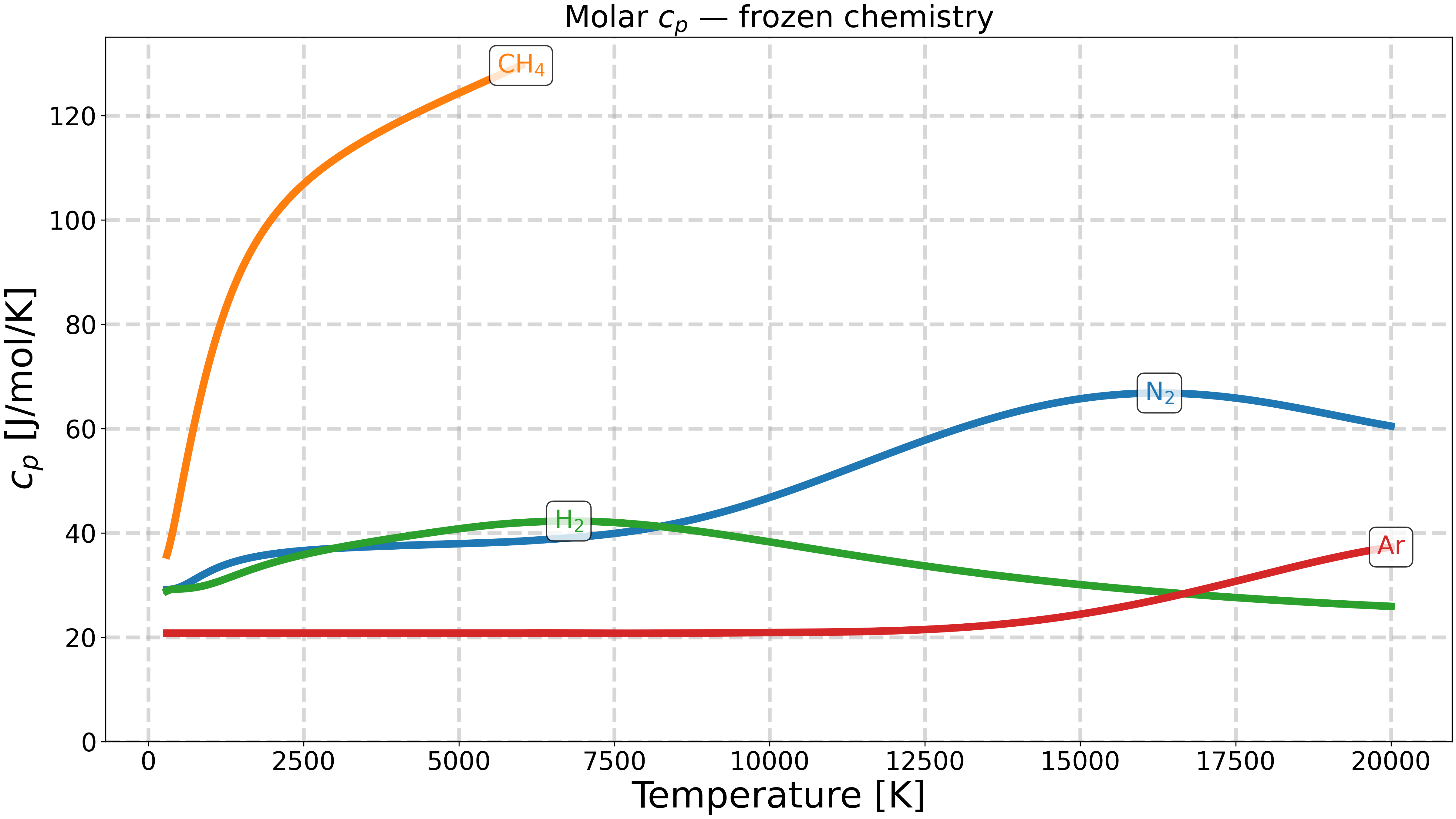
Total running time of the script: (0 minutes 4.408 seconds)