—

Time evolution of the formation of solid carbon in a hydrocarbon mixture.

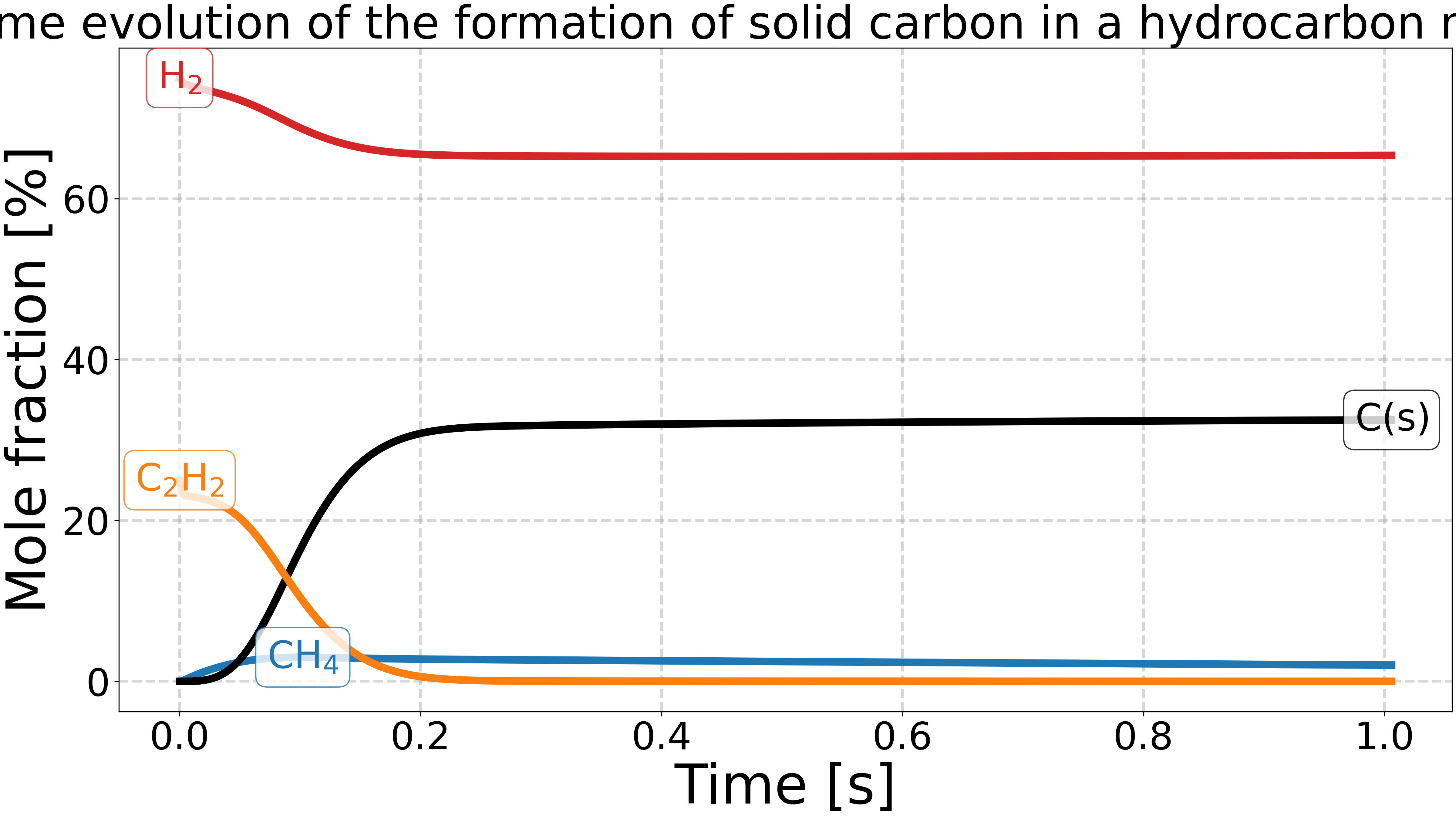
This example shows the time evolution of the formation of solid carbon in a hydrocarbon mixture.

The mechanism used is the Fincke GRC mechanism, which includes solid carbon (C(s)).

Thermodynamic data comes from [GRCDatabase] and [Burcat].

The initial composition is a hydrocarbon mixture, with a mole fraction of either 100 % methane, or 75 % acetylene and 25 % hydrogen.

The temperature is set constant at 1300 °C and the pressure is constant at 1 atm.

Tags: kinetics solid carbon formation

Import the required libraries.

import cantera as ct
import matplotlib.pyplot as plt
import numpy as np

from rizer.misc.plt_utils import (
    get_species_color,
    get_species_in_latex,
    get_text,
    set_mpl_style,
)
from rizer.misc.utils import get_path_to_data

set_mpl_style(nb_columns=1)

Define the parameters for the plot.

# Final time of the simulation.
final_time = 1  # s

# Species to plot.
species_to_plot = ["CH4", "H2", "C(s)", "C2H2"]

# Constant pressure of the reactor.
pressure = ct.one_atm

# Constant temperature of the reactor.
temperature = 1300 + 273.15  # K

# Initial composition of the reactor.
initial_composition = {"CH4": 0.0, "C2H2": 0.25, "H2": 0.75}

# Load Fincke GRC mechanism with soot carbon.
gas = ct.Solution(
    get_path_to_data("mechanisms", "Fincke_GRC.yaml"), name="gas_with_soot"
)

Compute time evolution of the formation of solid carbon.

# Set the initial conditions.
gas.TPX = temperature, pressure, initial_composition
# Create a constant pressure reactor.
reactor = ct.IdealGasConstPressureReactor(gas, energy="off", clone=False)
reactor_network = ct.ReactorNet([reactor])

# Store the states in a SolutionArray.
states = ct.SolutionArray(gas, 1, extra={"t": [0.0]})

# Run the simulation.
while reactor_network.time < final_time:
    reactor_network.step()
    states.append(gas.state, t=reactor_network.time)

Plot the results.

fig, ax = plt.subplots()
for species in species_to_plot:
    t = states.t  # type: ignore
    X = states(species).X * 100
    ax.plot(t, X, color=get_species_color(species))
    get_text(
        t[np.argmax(X)],
        X[np.argmax(X)],
        get_species_in_latex(species),
        ax=ax,
        color=get_species_color(species),
    )

ax.set_title("Time evolution of the formation of solid carbon in a hydrocarbon mixture")
ax.set_xlabel("Time [s]")
ax.set_ylabel("Mole fraction [%]")

plt.show()