—

Tutorial 3 — Loop inductance from the current rise into a dummy load.

What you measure: the load voltage (or current) with a known low-resistance dummy load (\(R_L \ll Z_0\), standing in for a spark) and a pulse much longer than the cable round trip.

What you calibrate: the series loop inductance the microsecond-scale model needs (e.g. wire_inductance of rizer’s RLRCircuit block). In this regime the whole line collapses into a series inductor — the Taylor expansion of the bounce recursion [Branin1967tdr] gives

\[L_{eff} = (R_g - Z_0)(R_L - Z_0)\,\frac{\ell}{Z_0 v} \;\xrightarrow{R_g, R_L \ll Z_0}\; L_{tot} = Z_0\,\ell/v ,\]

and the current rises exponentially with \(\tau_{LR} = L/(R_g+R_L)\).

Recipe.

1. Terminate with a known \(R_L\) (a few ohm, non-inductive), drive a flat-top pulse with \(T \gg 2\ell/v\), record \(V_L(t)\).

2. Fit the rise: \(V_L(t) = V_\infty (1 - e^{-t/\tau_{LR}})\) (a log-linear fit of \(1 - V_L/V_\infty\)).

3. \(L_{meas} = \tau_{LR}\,(R_g + R_L)\).

4. Compare with the cable’s own \(Z_0\ell/v\) from Tutorial 2: the surplus is the stray inductance of everything else in the loop (leads, electrode geometry) — that surplus is what belongs in the lumped circuit block on top of the cable.

Pitfalls: the fit is only valid past a few round trips (the staircase region); an inductive dummy load biases \(L\) up; too short a pulse never reaches \(V_\infty\) (the sweep at the end shows how long is long enough).

Tags: electric circuit transmission line inductance calibration tutorial

import matplotlib.pyplot as plt
import numpy as np

from rizer.electric_circuit.cable import IdealCable
from rizer.electric_circuit.generator import TrapezoidalGenerator
from rizer.electric_circuit.nrp_circuit import NRPCircuit

LENGTH, Z0, V_WAVE = 6.2, 75.0, 1.9e8
TAU_RT = 2 * LENGTH / V_WAVE
R_G, R_L, U_ON = 1.0, 2.0, 10e3
L_EFF = (R_G - Z0) * (R_L - Z0) * LENGTH / (Z0 * V_WAVE)


def march_line(t_pulse, r_l=R_L, r_g=R_G):
    """Play the 'measurement': wave-model line, trapezoid, resistive load."""
    gen = TrapezoidalGenerator(
        R_g=r_g,
        U_off=0.0,
        U_on=U_ON,
        t_rise=0.1 * t_pulse,
        t_on=0.8 * t_pulse,
        t_fall=0.1 * t_pulse,
    )
    line = NRPCircuit(gen, IdealCable(L=LENGTH, Z_c=Z0, c=V_WAVE))
    dt = min(TAU_RT / 200, t_pulse / 600)
    t = np.arange(dt, 1.6 * t_pulse + 6 * TAU_RT, dt)
    v_l = np.array(
        [line.compute_plasma_voltage(float(tk), R_p=r_l, nb_reflections=1) for tk in t]
    )
    v_g = np.array([gen.generator_voltage(float(tk)) for tk in t])
    return t, v_l, v_g


def march_lumped_rl(t, v_g, l_eff, r_l=R_L, r_g=R_G):
    """Evaluate the lumped series R-L model with the calibrated inductance."""
    i, r = 0.0, r_g + r_l
    decay = np.exp(-r * (t[1] - t[0]) / l_eff)
    v_l = np.empty_like(v_g)
    for k, vg in enumerate(v_g):
        i = i * decay + (vg / r) * (1.0 - decay)
        v_l[k] = r_l * i
    return v_l

Steps 1-3: the calibration shot and the exponential fit.

T_CAL = 10e-6
t, v_meas, v_g = march_line(T_CAL)

# Fit window: past the staircase (> 5 round trips), on the flat top.
v_inf = v_g * R_L / (R_G + R_L)  # the DC-divider asymptote
window = (t > 5 * TAU_RT) & (t < 0.6 * T_CAL) & (v_inf > 0.9 * v_inf.max())
residual = 1.0 - v_meas[window] / v_inf[window]
keep = residual > 1e-3
slope = np.polyfit(t[window][keep], np.log(residual[keep]), 1)[0]
tau_lr = -1.0 / slope
l_meas = tau_lr * (R_G + R_L)

print(f"fitted rise time  tau_LR = {tau_lr * 1e6:.2f} us")
print(f"L_meas = tau_LR (Rg+RL)  = {l_meas * 1e6:.2f} uH")
print(f"cable alone Z0 l / v     = {Z0 * LENGTH / V_WAVE * 1e6:.2f} uH")
print(f"matched-model L_eff      = {L_EFF * 1e6:.2f} uH")
print("surplus over the cable = stray loop inductance for the lumped block")

fig, ax = plt.subplots(figsize=(7, 4))
ax.plot(t * 1e6, v_meas / 1e3, lw=1.4, label="measured $V_L$ (wave model)")
ax.plot(
    t * 1e6,
    march_lumped_rl(t, v_g, l_meas) / 1e3,
    "--",
    lw=1.4,
    label=rf"R-L fit: $L$ = {l_meas * 1e6:.2f} $\mu$H",
)
ax.plot(t * 1e6, v_inf / 1e3, ":", lw=1.0, color="gray", label="DC divider")
ax.set_xlabel("t [us]")
ax.set_ylabel(r"$V_L$ [kV]")
ax.set_title("Calibration shot: fit the $L/R$ rise on the flat top")
ax.grid(alpha=0.3)
ax.legend(fontsize=9)
fig.tight_layout()
plt.show()

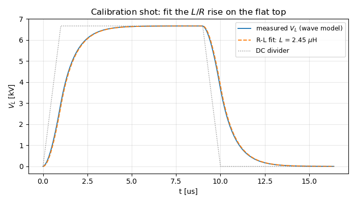
fitted rise time  tau_LR = 0.82 us
L_meas = tau_LR (Rg+RL)  = 2.45 uH
cable alone Z0 l / v     = 2.45 uH
matched-model L_eff      = 2.35 uH
surplus over the cable = stray loop inductance for the lumped block

How long is long enough? Below a few round trips the response is a reflection staircase and the L/R fit is meaningless; the deviation from the lumped model falls as tau/T (first order in the delay).

durations = [20e-9, 100e-9, 500e-9, 2e-6, 10e-6]
fig, axes = plt.subplots(1, len(durations), figsize=(17, 3.2), sharey=True)
errors = []
for ax, t_pulse in zip(axes, durations):
    t, v_wave, v_g = march_line(t_pulse)
    v_rl = march_lumped_rl(t, v_g, L_EFF)
    scale, unit = (1e9, "ns") if t_pulse < 1e-6 else (1e6, "us")
    ax.plot(t * scale, v_wave / 1e3, "-", lw=1.4, label="line")
    ax.plot(t * scale, v_rl / 1e3, "--", lw=1.4, label="lumped R-L")
    ax.set_title(f"T = {t_pulse * 1e9:g} ns  (T/τ = {t_pulse / TAU_RT:.1f})")
    ax.set_xlabel(f"t [{unit}]")
    ax.grid(alpha=0.3)
    errors.append(np.max(np.abs(v_wave - v_rl)) / np.max(np.abs(v_wave)))
axes[0].set_ylabel(r"$V_L$ [kV]")
axes[0].legend(fontsize=8)
fig.suptitle("Validity of the lumped fit: use pulses of many round trips", y=1.04)
fig.tight_layout()
plt.show()

for t_pulse, e in zip(durations, errors):
    print(f"T/tau = {t_pulse / TAU_RT:7.1f}   lumped-model deviation = {e:.3f}")

T/tau =     0.3   lumped-model deviation = 0.983
T/tau =     1.5   lumped-model deviation = 0.476
T/tau =     7.7   lumped-model deviation = 0.106
T/tau =    30.6   lumped-model deviation = 0.041
T/tau =   153.2   lumped-model deviation = 0.012

References

[Branin1967tdr]

F. H. Branin, “Transient analysis of lossless transmission lines,” Proc. IEEE 55(11), 2012-2013, 1967.