—
Elenbaas-Heller model for H₂ DC plasma — Cantera numerical solver.#
This example demonstrates how to use the Cantera-based numerical solver
(ThermalPlasmaColumn) to
compute the radial temperature profile of a DC plasma arc, and compares it
with the analytical Elenbaas-Heller solution.
The numerical model solves the same steady radial energy equation as the
analytical model but without the piecewise-linear \(\sigma(\Theta)\)
closure: it uses the full tabulated \(\sigma(T)\) and \(\kappa(T)\)
profiles from the LTE data, discretized on an adaptive radial grid via
Cantera’s Newton solver (rizer.cantera_ext._plasma1d extension).
This example requires the rizer-cantera conda environment:
conda activate rizer-cantera
Notes#
The Elenbaas-Heller equation in radial symmetry reads
where:
\(r\) is the radial distance [m],
\(\kappa(T)\) is the thermal conductivity [W/(m·K)],
\(\sigma(T)\) is the electrical conductivity [S/m],
\(E\) is the axial electric field [V/m],
\(P^{\mathrm{rad}}(T)\) is the radiative power density [W/m³].
The boundary conditions are:
\(T(R) = T_{\mathrm{wall}}\) (cooled wall),
\(dT/dr\,(r=0) = 0\) (axial symmetry).
The numerical solver discretizes this equation on a radial grid and refines it adaptively until the residuals are below the convergence threshold.
See Also#
Import the required libraries.#
import matplotlib.pyplot as plt
import numpy as np

from rizer.cantera_ext.thermal_plasma_column import ThermalPlasmaColumn
from rizer.misc.plt_utils import set_mpl_style
from rizer.thermal_plasma.elenbaas_heller import ElenbaasHeller
from rizer.thermal_plasma.fit_LTE_data import FitLTEData

set_mpl_style(nb_columns=1)
Load LTE transport data for hydrogen at 1 atm.#
H2_lte_data = FitLTEData(
    gas_name_transport="H2",
    gas_name_radiation="H2",
    pressure_atm=1,
    source_transport="Boulos2023",
    source_radiation="Gueye2017",
    emission_radius_mm=10,
    max_temperature_fit=12000.0,
)
/home/runner/work/rizer/rizer/rizer/thermal_plasma/fit_LTE_data.py:393: UserWarning: In `FitLTEData.fit_nec`, using previously fitted theta_sigma.
  warn("In `FitLTEData.fit_nec`, using previously fitted theta_sigma.")
Define common parameters.#
Solve with the analytical Elenbaas-Heller model.#
elenbaas = ElenbaasHeller(
    R,
    electric_field=None,
    current=current,
    gas_data=H2_lte_data,
)

print(f"Analytical — electric field: {elenbaas.electric_field:.2f} V/m")
print(f"Analytical — current:        {elenbaas.analytical_current():.2f} A")
Analytical — electric field: 4357.07 V/m
Analytical — current:        20.00 A
Solve with the Cantera numerical solver (no radiation).#
ThermalPlasmaColumn
accepts the same R, electric_field/current and gas_data
arguments as ElenbaasHeller.
column = ThermalPlasmaColumn(
    R,
    electric_field=None,
    current=current,
    gas_data=H2_lte_data,
    with_radiation=False,
)

print(f"Cantera     — electric field: {column.electric_field:.2f} V/m")
print(f"Cantera     — current:        {column.current():.2f} A")
print(f"Cantera     — grid points:    {column.n_points}")
/home/runner/work/rizer/rizer/rizer/thermal_plasma/elenbaas_heller.py:434: RuntimeWarning: The iteration is not making good progress, as measured by the
 improvement from the last ten iterations.
  temperature = fsolve(f, initial_temperature)[0]
Cantera     — electric field: 4442.05 V/m
Cantera     — current:        20.01 A
Cantera     — grid points:    108
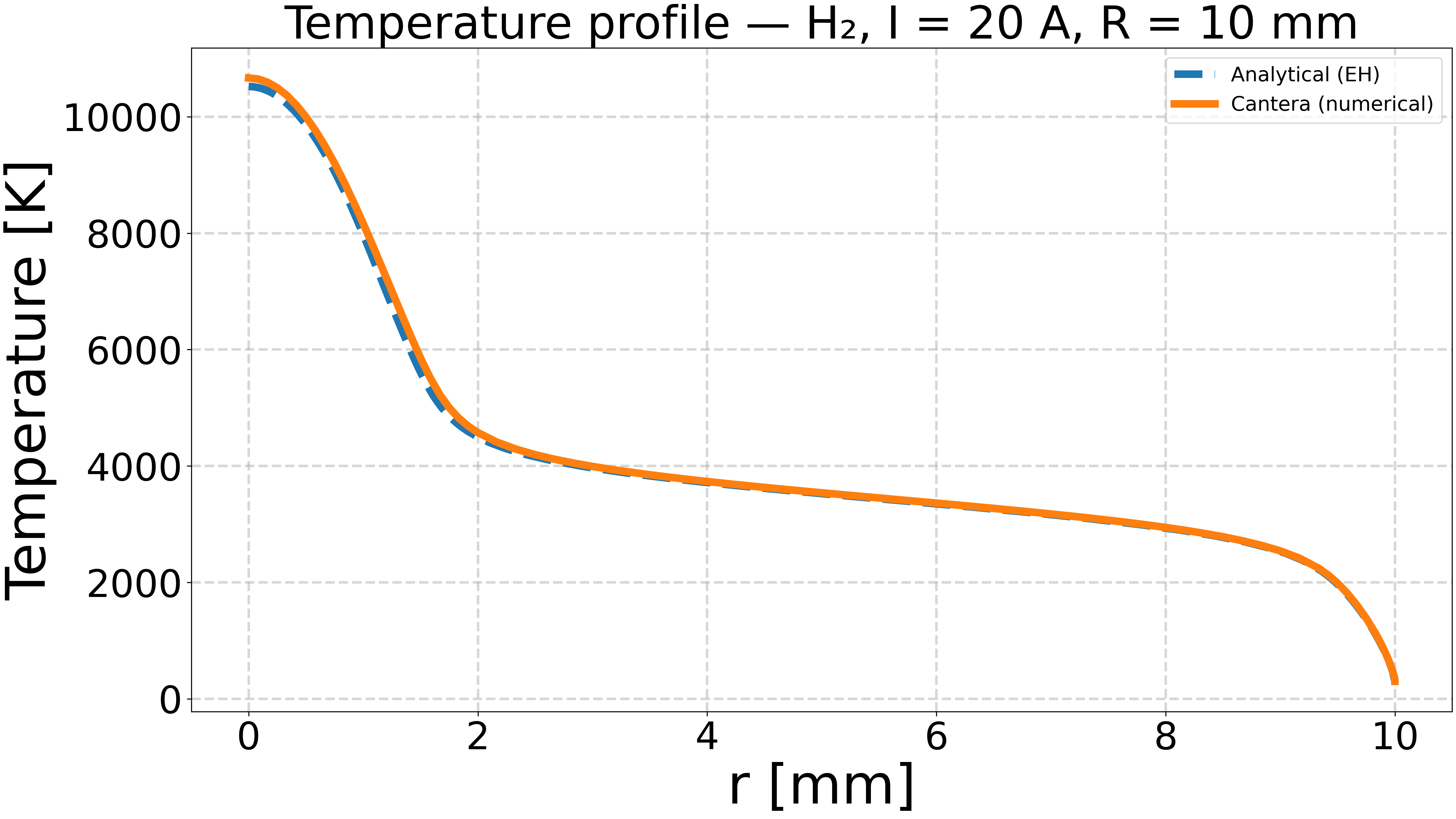
Compare temperature profiles.#
Plot the analytical and numerical temperature profiles side by side. The two should agree closely; any difference reflects the linearised \(\sigma(\Theta)\) approximation used by the analytical model.
r_dense = np.linspace(0, R, 500)
T_analytical = np.array([elenbaas.get_temperature_vs_radius(r) for r in r_dense])

r_num, T_num = column.temperature_profile()

fig, ax = plt.subplots()
ax.plot(r_dense * 1e3, T_analytical, label="Analytical (EH)", linestyle="--")
ax.plot(r_num * 1e3, T_num, label="Cantera (numerical)", linestyle="-")
ax.set_xlabel("r [mm]")
ax.set_ylabel("Temperature [K]")
ax.set_title(f"Temperature profile — H₂, I = {current} A, R = {R * 1e3:.0f} mm")
ax.legend()
plt.show()
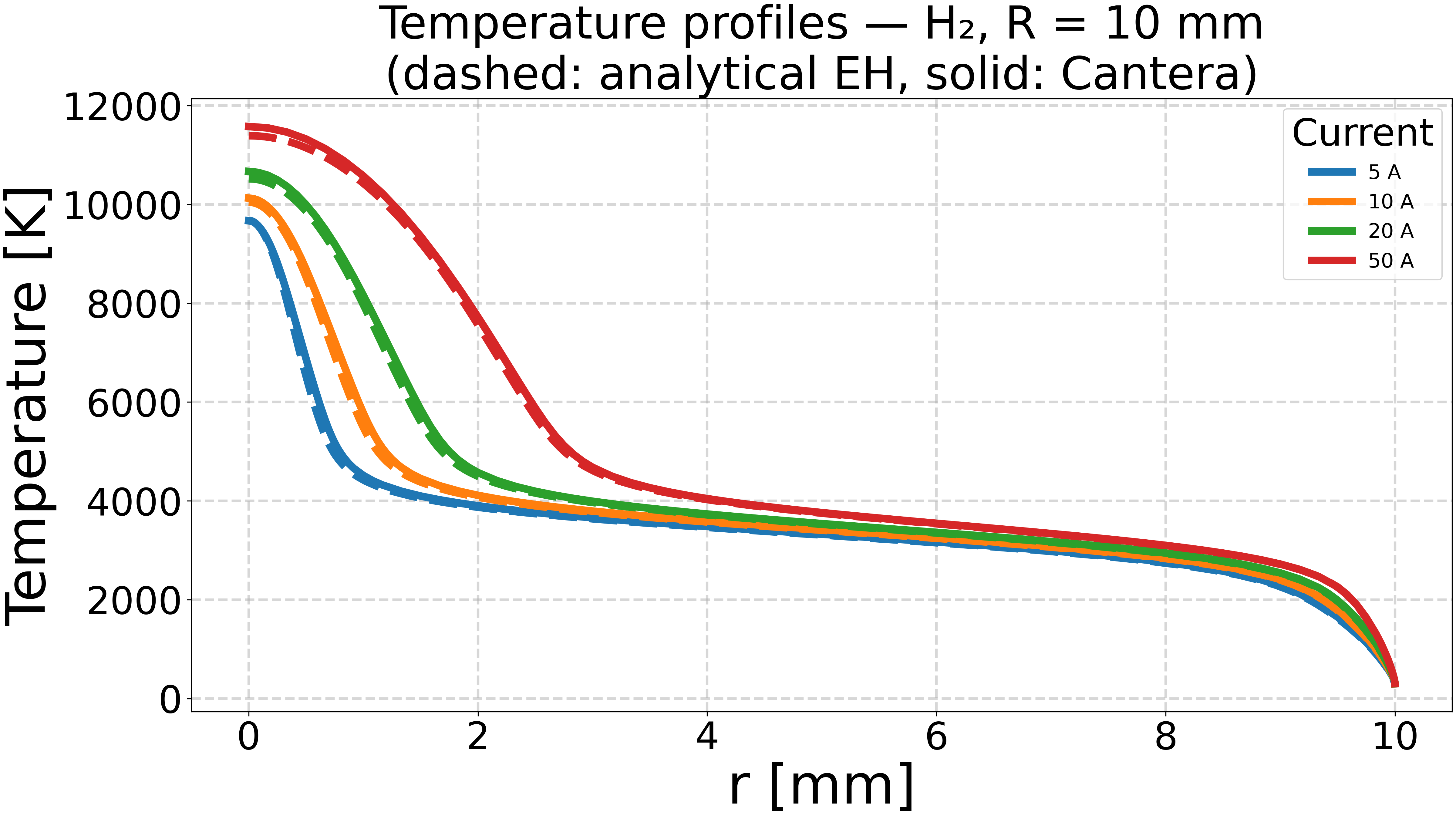
Sweep over multiple current values.#
Compare the analytical and numerical temperature profiles for several arc currents to assess how the linearised closure affects the prediction at different power levels.
currents = [5, 10, 20, 50]  # A

fig, ax = plt.subplots()

for current in currents:
    eh = ElenbaasHeller(R, electric_field=None, current=current, gas_data=H2_lte_data)
    col = ThermalPlasmaColumn(
        R,
        electric_field=None,
        current=current,
        gas_data=H2_lte_data,
        with_radiation=False,
    )

    T_eh = np.array([eh.get_temperature_vs_radius(r) for r in r_dense])
    r_c, T_c = col.temperature_profile()

    # Plot numerical first to consume a color, then reuse it for the analytical line.
    (line,) = ax.plot(r_c * 1e3, T_c, linestyle="-", label=f"{current} A")
    ax.plot(r_dense * 1e3, T_eh, linestyle="--", color=line.get_color())

# Add a legend for current values and a note about line styles.
handles, labels = ax.get_legend_handles_labels()
ax.legend(handles, labels, title="Current")
ax.set_xlabel("r [mm]")
ax.set_ylabel("Temperature [K]")
ax.set_title(
    f"Temperature profiles — H₂, R = {R * 1e3:.0f} mm\n"
    "(dashed: analytical EH, solid: Cantera)"
)
plt.show()
Effect of radiation on the temperature profile.#
The Cantera solver supports including the radiative sink \(P^{\mathrm{rad}}(T) = 4\pi\,\mathrm{NEC}(T)\) directly. Compare without and with radiation for a single operating point.
I_rad = 170  # A — radiation effects are more visible at high power

col_no_rad = ThermalPlasmaColumn(
    R,
    electric_field=None,
    current=I_rad,
    gas_data=H2_lte_data,
    with_radiation=False,
)

col_rad = ThermalPlasmaColumn(
    R,
    electric_field=None,
    current=I_rad,
    gas_data=H2_lte_data,
    with_radiation=True,
)

r_nr, T_nr = col_no_rad.temperature_profile()
r_wr, T_wr = col_rad.temperature_profile()

fig, ax = plt.subplots()
ax.plot(r_nr * 1e3, T_nr, label="Without radiation")
ax.plot(r_wr * 1e3, T_wr, label="With radiation")
ax.set_xlabel("r [mm]")
ax.set_ylabel("Temperature [K]")
ax.set_title(f"Radiation effect — H₂, I = {I_rad} A, R = {R * 1e3:.0f} mm")
ax.legend()
plt.show()

Numerical vs. analytical, with radiation.#
The analytical Elenbaas-Heller model also supports radiation
(with_radiation=True): the net emission coefficient is linearized about
\(\theta_\sigma\) just like \(\sigma\), so the arc-channel parameter
becomes \(\epsilon = \sqrt{a_\sigma E^2 - b}\) with \(b = 4\pi a_\varepsilon\).
Both models then solve the same radiative balance, the analytical one with the
linearized closure and the numerical one with the full tabulated properties.
We compare them at a fixed electric field (current control with radiation can be non-monotonic in \(E\), so a fixed field gives a clean apples-to-apples comparison).
E_cmp = 5000  # V/m

# Analytical model with radiation, at fixed E.
elenbaas_rad = ElenbaasHeller(
    R, electric_field=E_cmp, gas_data=H2_lte_data, with_radiation=True
)
T_analytical_rad = np.array(
    [elenbaas_rad.get_temperature_vs_radius(r) for r in r_dense]
)

# Numerical model with radiation, at the same fixed E.
col_cmp = ThermalPlasmaColumn(
    R, electric_field=E_cmp, gas_data=H2_lte_data, with_radiation=True
)
r_cmp, T_cmp = col_cmp.temperature_profile()

print(f"With radiation, E = {E_cmp} V/m:")
print(
    f"  Analytical — T_center: {elenbaas_rad.get_temperature_vs_radius(0.0):.1f} K, "
    f"current: {elenbaas_rad.analytical_current():.2f} A"
)
print(
    f"  Cantera    — T_center: {col_cmp.get_temperature_vs_radius(0.0):.1f} K, "
    f"current: {col_cmp.current():.2f} A"
)

fig, ax = plt.subplots()
ax.plot(r_dense * 1e3, T_analytical_rad, "--", label="Analytical (EH + radiation)")
ax.plot(r_cmp * 1e3, T_cmp, "-", label="Cantera (numerical + radiation)")
ax.set_xlabel("r [mm]")
ax.set_ylabel("Temperature [K]")
ax.set_title(
    f"Numerical vs. analytical with radiation — H₂, E = {E_cmp} V/m, "
    f"R = {R * 1e3:.0f} mm"
)
ax.legend()
plt.show()
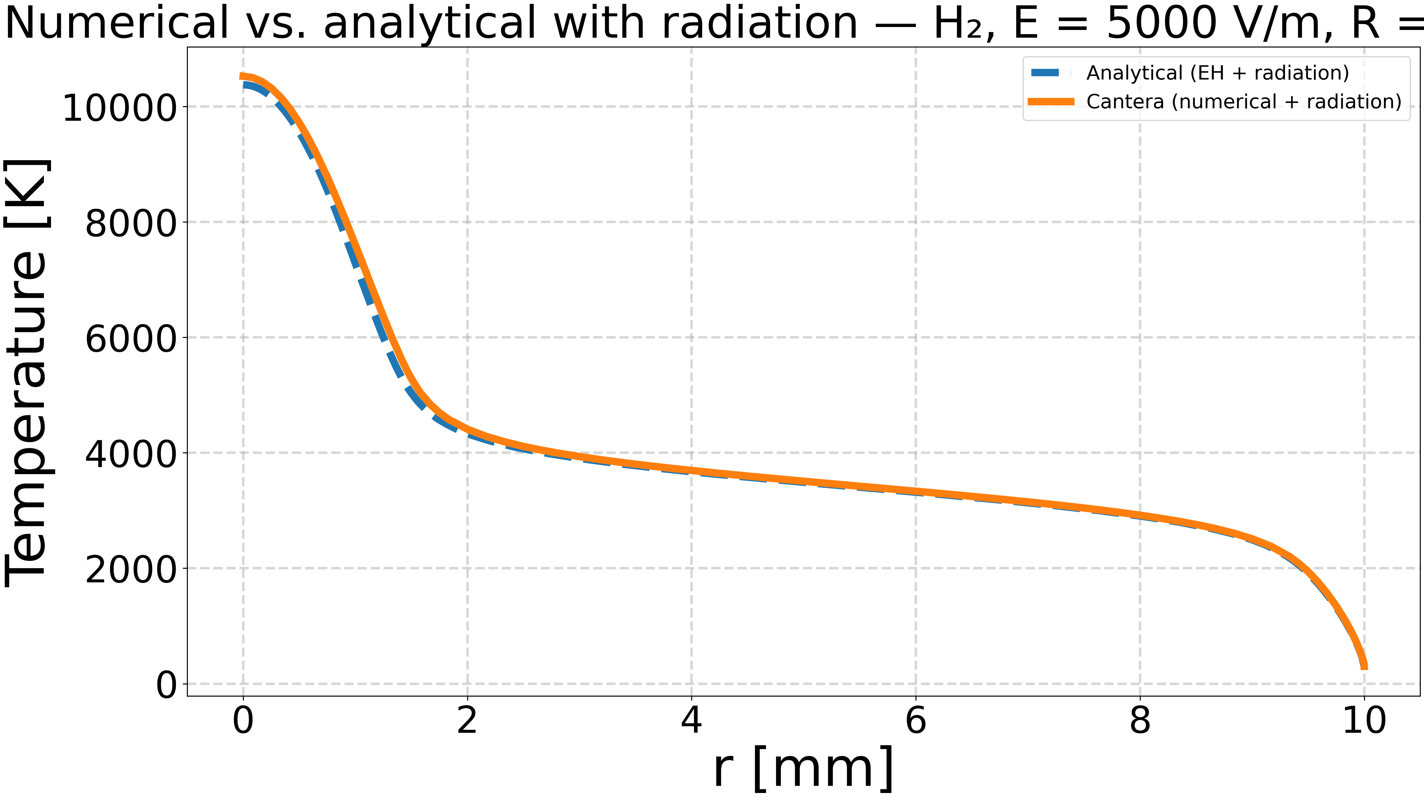
With radiation, E = 5000 V/m:
  Analytical — T_center: 10377.4 K, current: 16.65 A
  Cantera    — T_center: 10525.5 K, current: 16.94 A
Total running time of the script: (0 minutes 2.484 seconds)