—

Tutorial 2 — TDR: calibrate the cable delay and impedance from echoes.

What you measure: the voltage at the generator end of the cable with a fast step, for three far-end terminations: open, short, and a known resistor. This is time-domain reflectometry (TDR) [Johnson1993].

What you calibrate:

• the round-trip delay \(\tau = 2\ell/v\) — the time between the launched edge and the first echo. With the cable length known this gives the wave speed \(v\) (and hence the transit time the retarded-time circuit model needs); with the cable type known it measures \(\ell\).

• the characteristic impedance \(Z_0\) — from the echo amplitude. The first echo returns a fraction \((1+\Gamma_g)\,\Gamma_L\) of the launched step, with \(\Gamma = (R - Z_0)/(R + Z_0)\) at each end: an open end (\(\Gamma_L = +1\)) steps up, a short (\(\Gamma_L = -1\)) steps down, and a termination with a known resistor lets you solve \(Z_0 = R\,(1-\Gamma_L)/(1+\Gamma_L)\) from the measured ratio.

Recipe.

1. Terminate the far end (open, then short, then known R), drive a step much faster than \(\tau\), record \(V(t)\) at the generator end.

2. \(\Delta t(\text{edge} \to \text{first echo}) = 2\ell/v\).

3. First-echo amplitude / launched amplitude \(= (1+\Gamma_g)\Gamma_L\); with the open trace this yields \(\Gamma_g\) (hence \(Z_0\) if \(R_g\) is known, or vice versa); the known-R trace cross-checks.

4. Feed \(\ell\), \(v\) (wave speed), \(Z_c\) into the Cable block / electric_circuit.cable section of the rizer configuration.

Pitfalls: a slow source edge smears the echo (keep rise time \(\ll \tau\)); resistive cable losses tilt the plateaus; probe capacitance rounds the steps.

Tags: electric circuit transmission line TDR calibration tutorial

import matplotlib.pyplot as plt
import numpy as np

# The cable under test (the NRP example cable).
LENGTH, Z0, V_WAVE = 6.2, 75.0, 1.9e8
TAU_RT = 2 * LENGTH / V_WAVE
R_G = 25.0  # generator internal resistance (deliberately unmatched)
U_STEP = 1.0  # normalized step amplitude
T_RISE = 2e-9


def v_generator_end(t, r_load, n_echoes=12):
    """Voltage at the generator end of the line (bounce-sum, frozen load).

    The launched wave is V_g * Z0/(R_g+Z0); each round trip returns it
    scaled by Gamma_L * Gamma_g per bounce, and an arriving wave deposits
    (1 + Gamma_g) times its amplitude at the source end.
    """
    gamma_g = (R_G - Z0) / (R_G + Z0)
    gamma_l = (r_load - Z0) / (r_load + Z0) if np.isfinite(r_load) else 1.0
    launch = Z0 / (R_G + Z0)

    def step(x):  # the source edge, linear ramp of T_RISE
        return U_STEP * np.clip(x / T_RISE, 0.0, 1.0)

    v = launch * step(t)
    for k in range(1, n_echoes + 1):
        v = v + launch * (1 + gamma_g) * gamma_l**k * gamma_g ** (k - 1) * step(
            t - k * TAU_RT
        )
    return v

The three calibration traces.

t = np.linspace(0.0, 5.5 * TAU_RT, 4000)
cases = [
    ("open", np.inf, "tab:blue"),
    ("short", 1e-9, "tab:red"),
    ("known R = 150 ohm", 150.0, "tab:green"),
]

fig, ax = plt.subplots(figsize=(8, 4.5))
for label, r_load, color in cases:
    ax.plot(t * 1e9, v_generator_end(t, r_load), color=color, lw=1.5, label=label)
for k in range(1, 6):
    ax.axvline(k * TAU_RT * 1e9, color="gray", ls=":", lw=0.7)
ax.text(TAU_RT * 1e9, 0.02, r"  $\tau = 2\ell/v$", fontsize=9, color="gray")
ax.set_xlabel("t [ns]")
ax.set_ylabel(r"$V_{gen\ end}\,/\,V_{step}$")
ax.set_title("TDR at the generator end: echo timing -> delay, echo amplitude -> $Z_0$")
ax.grid(alpha=0.3)
ax.legend(fontsize=9)
fig.tight_layout()
plt.show()

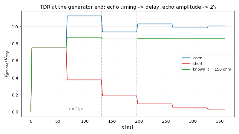
Extract the calibration numbers as an experimenter would.

launch = Z0 / (R_G + Z0)
gamma_g = (R_G - Z0) / (R_G + Z0)

v_open = v_generator_end(t, np.inf)
edge_lvl = launch * U_STEP
i_echo = np.argmax(v_open > edge_lvl * 1.02)  # first departure from the plateau
tau_measured = t[i_echo]
print(
    f"measured first-echo delay : {tau_measured * 1e9:6.1f} ns "
    f"(true 2 l/v = {TAU_RT * 1e9:.1f} ns)"
)
print(
    f"-> wave speed v = 2 l / dt = {2 * LENGTH / tau_measured:.3g} m/s "
    f"(true {V_WAVE:.3g})"
)

# Echo amplitude on the open trace: (1 + Gamma_g) * 1.
plateau_1 = v_open[(t > 1.2 * TAU_RT) & (t < 1.8 * TAU_RT)].mean()
ratio = (plateau_1 - edge_lvl) / edge_lvl
gamma_g_measured = ratio - 1.0
z0_measured = R_G * (1 - gamma_g_measured) / (1 + gamma_g_measured)
print(f"open-end echo ratio       : {ratio:6.3f} = 1 + Gamma_g")
print(f"-> Z0 = R_g (1-G)/(1+G)   = {z0_measured:6.1f} ohm (true {Z0:.1f})")

measured first-echo delay :   65.3 ns (true 2 l/v = 65.3 ns)
-> wave speed v = 2 l / dt = 1.9e+08 m/s (true 1.9e+08)
open-end echo ratio       :  0.500 = 1 + Gamma_g
-> Z0 = R_g (1-G)/(1+G)   =   75.0 ohm (true 75.0)

References

[Johnson1993]

H. W. Johnson, M. Graham, High-Speed Digital Design, Prentice Hall, 1993 (TDR and transmission-line measurement practice).