—

Tutorial 4 — Cable capacitance from the charging transient (no load).

What you measure: the far-end voltage with the load disconnected (or a known high resistance \(R_L \gg Z_0\)) and a known series source resistance.

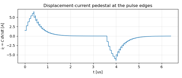
What you calibrate: the cable’s total shunt capacitance \(C_{tot} = \ell/(Z_0 v)\) — the open-stub limit \(Z_{in} \to 1/(j\omega C_{tot})\) [Pozar2011cap]. This is the capacitance that produces the displacement-current spike your current probe sees at every pulse edge even with no discharge burning; calibrating it lets you subtract that pedestal from measured discharge currents.

Recipe.

1. Open the far end (or terminate with a known \(R_L \gg Z_0\)); insert a known resistor \(R_g\) at the source (large enough that \(R_g C_{tot}\) spans several cable round trips).

2. Record \(V_L(t)\) for a flat-top pulse; fit the exponential charge \(V_L = V_\infty(1 - e^{-t/\tau_{RC}})\).

3. \(C_{meas} = \tau_{RC} / (R_g \,\|\, R_L)\); cross-check against the datasheet \(C' \approx 70\text{-}100\) pF/m for typical coax.

4. Use it to predict the edge current spike \(i_C = C_{tot}\,dV/dt\) and subtract it from discharge current measurements.

Pitfalls: probe input capacitance adds directly to \(C_{meas}\) (calibrate the probe first or subtract it); a leaky “open” (humidity, probe resistance) turns the plateau into a slow droop.

Tags: electric circuit transmission line capacitance calibration tutorial

import matplotlib.pyplot as plt
import numpy as np

from rizer.electric_circuit.cable import IdealCable
from rizer.electric_circuit.generator import TrapezoidalGenerator
from rizer.electric_circuit.nrp_circuit import NRPCircuit

LENGTH, Z0, V_WAVE = 6.2, 75.0, 1.9e8
TAU_RT = 2 * LENGTH / V_WAVE
C_TOT = LENGTH / (Z0 * V_WAVE)
R_G, R_L, U_ON = 1000.0, 5000.0, 10e3
T_PULSE = 4e-6

The ‘measurement’: wave model with a high-impedance termination.

gen = TrapezoidalGenerator(
    R_g=R_G,
    U_off=0.0,
    U_on=U_ON,
    t_rise=0.1 * T_PULSE,
    t_on=0.8 * T_PULSE,
    t_fall=0.1 * T_PULSE,
)
line = NRPCircuit(gen, IdealCable(L=LENGTH, Z_c=Z0, c=V_WAVE))
dt = TAU_RT / 200
t = np.arange(dt, 1.6 * T_PULSE, dt)
v_meas = np.array(
    [line.compute_plasma_voltage(float(tk), R_p=R_L, nb_reflections=1) for tk in t]
)
v_g = np.array([gen.generator_voltage(float(tk)) for tk in t])

Steps 2-3: fit the RC charge on the flat top and recover C.

v_inf = v_g * R_L / (R_G + R_L)
window = (t > 5 * TAU_RT) & (t < 0.55 * T_PULSE) & (v_inf > 0.9 * v_inf.max())
residual = 1.0 - v_meas[window] / v_inf[window]
keep = residual > 1e-3
slope = np.polyfit(t[window][keep], np.log(residual[keep]), 1)[0]
tau_rc = -1.0 / slope
r_parallel = 1.0 / (1.0 / R_G + 1.0 / R_L)
c_meas = tau_rc / r_parallel

print(f"fitted charge time tau_RC = {tau_rc * 1e9:.0f} ns")
print(
    f"C_meas = tau_RC/(Rg||RL)  = {c_meas * 1e12:.0f} pF "
    f"(true C_tot = {C_TOT * 1e12:.0f} pF, "
    f"C' = {C_TOT / LENGTH * 1e12:.1f} pF/m)"
)

# Lumped RC prediction with the calibrated value.
g = 1.0 / R_G + 1.0 / R_L
decay = np.exp(-g * dt / c_meas)
v_rc, v = np.empty_like(v_g), 0.0
for k, vg in enumerate(v_g):
    v = v * decay + (vg / (R_G * g)) * (1.0 - decay)
    v_rc[k] = v

fig, ax = plt.subplots(figsize=(7, 4))
ax.plot(t * 1e6, v_meas / 1e3, "-", lw=1.4, label="measured $V_L$ (wave model)")
ax.plot(t * 1e6, v_rc / 1e3, "--", lw=1.4, label=f"R-C fit: C = {c_meas * 1e12:.0f} pF")
ax.plot(t * 1e6, v_inf / 1e3, ":", lw=1.0, color="gray", label="DC divider")
ax.set_xlabel("t [us]")
ax.set_ylabel(r"$V_L$ [kV]")
ax.set_title("Calibration shot: the open cable charges as one capacitor")
ax.grid(alpha=0.3)
ax.legend(fontsize=9)
fig.tight_layout()
plt.show()

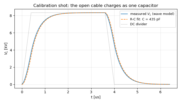
fitted charge time tau_RC = 362 ns
C_meas = tau_RC/(Rg||RL)  = 435 pF (true C_tot = 435 pF, C' = 70.2 pF/m)

The payoff for current measurements: the capacitive edge spike this calibrated C predicts (to be subtracted from discharge currents).

i_c = c_meas * np.gradient(v_meas, t)
fig, ax = plt.subplots(figsize=(7, 3))
ax.plot(t * 1e6, i_c, lw=1.2)
ax.set_xlabel("t [us]")
ax.set_ylabel(r"$i_C = C\,dV/dt$ [A]")
ax.set_title("Displacement-current pedestal at the pulse edges")
ax.grid(alpha=0.3)
fig.tight_layout()
plt.show()

References

[Pozar2011cap]

4. 13. Pozar, Microwave Engineering, 4th ed., Wiley, 2011, ch. 2.