—

Tutorial 1 — Electrical length: which circuit model does your setup need?

The decision this tutorial supports: before calibrating anything, decide whether your cabling must be modelled as a transmission line (rizer’s Cable block / NRPCircuit) or collapses into a lumped element (an RLRCircuit inductance, a stray capacitance) — because the answer decides which parameters exist to be calibrated.

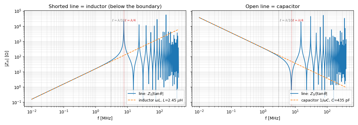
A transmission line of length \(\ell\) is “long” or “short” only relative to the wavelength: its electrical length is \(\theta = \omega\ell/v\). Below the classic \(\ell < \lambda/10\) criterion [Ulaby2015] (time-domain twin: rise time \(t_r \gtrsim 3.5\,\ell/v\)) the line is indistinguishable from a lumped element — which element depends on the termination, via the input-impedance formula [Pozar2011] (eq. 2.44):

\[\begin{split}Z_{in} = Z_0\,\frac{Z_L + jZ_0\tan\theta}{Z_0 + jZ_L\tan\theta} \;\xrightarrow{\;\theta \ll 1\;}\; \begin{cases} j\omega\,(Z_0\ell/v) & Z_L = 0 \text{ (shorted = inductor)}\\[4pt] 1/\bigl(j\omega\,\ell/(Z_0 v)\bigr) & Z_L \to \infty \text{ (open = capacitor)} \end{cases}\end{split}\]

so the inductance of a shorted line is its impedance times its delay, \(L_{tot} = Z_0\,T\). Above the boundary the line resonates at \(\ell = \lambda/4, \lambda/2, \dots\) — physics no lumped element has.

Rule of thumb for the lab: nanosecond NRP pulses on meters of coax are always distributed (calibrate \(Z_0\), \(\ell/v\): Tutorial 2); microsecond spark currents see a lumped \(L\) (Tutorial 3); edge spikes into an open line see a lumped \(C\) (Tutorial 4).

The specimen is the NRP example cable (6.2 m, 75 \(\Omega\), \(v = 1.9\times 10^8\) m/s); no plasma involved.

Tags: electric circuit transmission line electrical length tutorial

import matplotlib.pyplot as plt
import numpy as np

The cable and its per-unit-length parameters.

LENGTH = 6.2  # m
Z0 = 75.0  # ohm
V_WAVE = 1.9e8  # m/s

L_TOT = Z0 * LENGTH / V_WAVE  # shorted-line (series) inductance,  L' * l
C_TOT = LENGTH / (Z0 * V_WAVE)  # open-line (shunt) capacitance,     C' * l
print(f"L_tot = {L_TOT * 1e6:.2f} uH, C_tot = {C_TOT * 1e12:.0f} pF")
print(f"lumped below f = v/(10 l) = {V_WAVE / (10 * LENGTH) / 1e6:.2f} MHz")

L_tot = 2.45 uH, C_tot = 435 pF
lumped below f = v/(10 l) = 3.06 MHz

Input impedance vs frequency for the two extreme terminations, with the lumped-element overlays and the electrical-length landmarks.

f = np.logspace(4, 8.6, 2000)
w = 2 * np.pi * f
theta = w * LENGTH / V_WAVE
f_lumped = V_WAVE / (10 * LENGTH)
f_quarter = V_WAVE / (4 * LENGTH)

fig, axes = plt.subplots(1, 2, figsize=(12, 4.2), sharey=True)
axes[0].loglog(
    f / 1e6, Z0 * np.abs(np.tan(theta)), lw=1.5, label=r"line: $Z_0|\tan\theta|$"
)
axes[0].loglog(
    f / 1e6,
    w * L_TOT,
    "--",
    lw=1.3,
    label=rf"inductor $\omega L$, $L$={L_TOT * 1e6:.2f} $\mu$H",
)
axes[0].set_title("Shorted line = inductor (below the boundary)")
axes[1].loglog(
    f / 1e6, Z0 / np.abs(np.tan(theta)), lw=1.5, label=r"line: $Z_0/|\tan\theta|$"
)
axes[1].loglog(
    f / 1e6,
    1 / (w * C_TOT),
    "--",
    lw=1.3,
    label=rf"capacitor $1/\omega C$, $C$={C_TOT * 1e12:.0f} pF",
)
axes[1].set_title("Open line = capacitor")
for ax in axes:
    ax.axvline(f_lumped / 1e6, color="gray", ls=":", lw=1)
    ax.axvline(f_quarter / 1e6, color="tab:red", ls=":", lw=1)
    ax.text(f_lumped / 1e6, 2e4, r" $\ell=\lambda/10$", fontsize=8, color="gray")
    ax.text(f_quarter / 1e6, 2e4, r" $\ell=\lambda/4$", fontsize=8, color="tab:red")
    ax.set_xlabel("f [MHz]")
    ax.grid(alpha=0.3, which="both")
    ax.legend(fontsize=9, loc="lower right")
axes[0].set_ylabel(r"$|Z_{in}|$ [$\Omega$]")
fig.tight_layout()
plt.show()

References

[Pozar2011]

4. 13. Pozar, Microwave Engineering, 4th ed., Wiley, 2011, ch. 2.

[Ulaby2015]

F. T. Ulaby, U. Ravaioli, Fundamentals of Applied Electromagnetics, 7th ed., Pearson, 2015, ch. 2.