—

Tutorial 5 — The LC-ladder view: why the calibrations are consistent.

The conceptual capstone of the series: why the \(Z_0, v\) you measured by TDR (Tutorial 2) and the \(L\), \(C\) you fitted from slow transients (Tutorials 3-4) are the same two numbers in different clothes.

Discretize a line into \(N\) cells of series \(L' dz\) and shunt \(C' dz\) — the ladder from which the telegrapher’s equations are derived [Ramo1994] [Paul2008]. The link between \(L'\) and the total inductance seen at slow (microsecond) timescales is then just series addition:

\[L_{seen} = \sum_{k=1}^{N} L'\,dz = L'\ell = Z_0\,\ell/v = L_{tot},\]

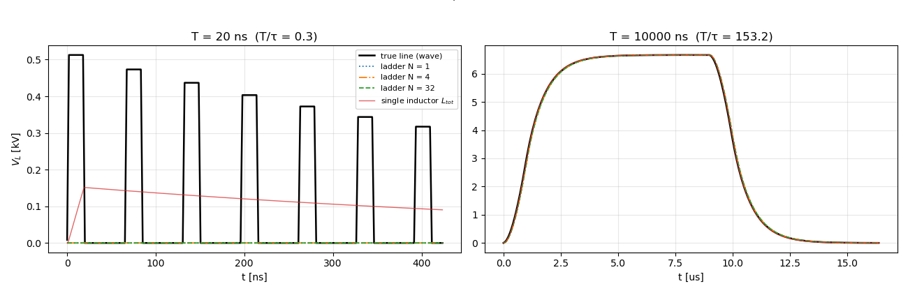
valid once the current is uniform along the line — series inductors only add when they carry the same current, and at slow timescales the shunt capacitors carry nothing, so all cells share one current. The sum is independent of \(N\): even a single cell gets the slow limit right. \(L'\) is therefore the density of the inductance you measure at the microsecond level.

For fast (nanosecond) signals the capacitors decouple the cells, the current differs cell to cell (that non-uniformity is the wavefront), and instead of adding inductances each cell contributes a delay \(\sqrt{L'dz\,C'dz} = dz/v\) — the ladder is a delay line (an artificial line / pulse-forming network). A finite ladder imitates the true line only below its per-cell cutoff \(f_c = N v/(\pi\ell)\), i.e. for roughly \(N \gtrsim 10\,\ell/\lambda_{min}\) sections. The wave regime is nothing but the transient during which the cells have not yet agreed on a common current.

The demo drives identical ladders (\(N = 1, 4, 32\)) with a 20 ns and a 10 us pulse: fast, they fan out and only \(N=32\) tracks the true wave solution; slow, all of them collapse onto the single-inductor curve.

Tags: electric circuit transmission line LC ladder inductance tutorial

import matplotlib.pyplot as plt
import numpy as np
from scipy.integrate import solve_ivp

from rizer.electric_circuit.cable import IdealCable
from rizer.electric_circuit.generator import TrapezoidalGenerator
from rizer.electric_circuit.nrp_circuit import NRPCircuit

LENGTH, Z0, V_WAVE = 6.2, 75.0, 1.9e8
TAU_RT = 2 * LENGTH / V_WAVE
L_TOT = Z0 * LENGTH / V_WAVE
C_TOT = LENGTH / (Z0 * V_WAVE)
R_G, R_L, U_ON = 1.0, 2.0, 10e3
L_EFF = (R_G - Z0) * (R_L - Z0) * LENGTH / (Z0 * V_WAVE)


def _generator(t_pulse):
    return TrapezoidalGenerator(
        R_g=R_G,
        U_off=0.0,
        U_on=U_ON,
        t_rise=0.1 * t_pulse,
        t_on=0.8 * t_pulse,
        t_fall=0.1 * t_pulse,
    )


def march_line(t_pulse):
    """Reference: the exact wave model (Branin recursion)."""
    gen = _generator(t_pulse)
    line = NRPCircuit(gen, IdealCable(L=LENGTH, Z_c=Z0, c=V_WAVE))
    dt = min(TAU_RT / 200, t_pulse / 600)
    t = np.arange(dt, 1.6 * t_pulse + 6 * TAU_RT, dt)
    v_l = np.array(
        [line.compute_plasma_voltage(float(tk), R_p=R_L, nb_reflections=1) for tk in t]
    )
    v_g = np.array([gen.generator_voltage(float(tk)) for tk in t])
    return t, v_l, v_g


def march_ladder(t_pulse, n_cells):
    """N-section LC ladder (series L' dz, shunt C' dz) into the load."""
    L_c, C_c = L_TOT / n_cells, C_TOT / n_cells
    gen = _generator(t_pulse)

    def rhs(t, y):
        i, v = y[:n_cells], y[n_cells:]
        vg = gen.generator_voltage(t)
        v_up = np.concatenate(([vg - R_G * i[0]], v[:-1]))
        di = (v_up - v) / L_c
        i_out = np.concatenate((i[1:], [v[-1] / R_L]))
        dv = (i - i_out) / C_c
        return np.concatenate((di, dv))

    t_end = 1.6 * t_pulse + 6 * TAU_RT
    t_eval = np.linspace(0.0, t_end, 1200)
    sol = solve_ivp(
        rhs, (0.0, t_end), np.zeros(2 * n_cells), t_eval=t_eval, rtol=1e-7, atol=1e-3
    )
    return sol.t, sol.y[-1]


def march_lumped_rl(t, v_g):
    """The single series inductor L_eff (exponential-step Euler)."""
    i, r = 0.0, R_G + R_L
    decay = np.exp(-r * (t[1] - t[0]) / L_EFF)
    v_l = np.empty_like(v_g)
    for k, vg in enumerate(v_g):
        i = i * decay + (vg / r) * (1.0 - decay)
        v_l[k] = R_L * i
    return v_l

Fast and slow drive of the same ladders.

fig, axes = plt.subplots(1, 2, figsize=(13, 4.2))
for ax, t_pulse in zip(axes, (20e-9, 10e-6)):
    t_w, v_w, v_g = march_line(t_pulse)
    scale, unit = (1e9, "ns") if t_pulse < 1e-6 else (1e6, "us")
    ax.plot(t_w * scale, v_w / 1e3, "k-", lw=1.8, label="true line (wave)")
    for n, style in ((1, ":"), (4, "-."), (32, "--")):
        t_l, v_l = march_ladder(t_pulse, n)
        ax.plot(t_l * scale, v_l / 1e3, style, lw=1.3, label=f"ladder N = {n}")
    ax.plot(
        t_w * scale,
        march_lumped_rl(t_w, v_g) / 1e3,
        lw=1.0,
        alpha=0.7,
        label=r"single inductor $L_{tot}$",
    )
    ax.set_title(f"T = {t_pulse * 1e9:g} ns  (T/τ = {t_pulse / TAU_RT:.1f})")
    ax.set_xlabel(f"t [{unit}]")
    ax.grid(alpha=0.3)
axes[0].set_ylabel(r"$V_L$ [kV]")
axes[0].legend(fontsize=8)
fig.suptitle("The same LC ladders, driven fast and slow", y=1.03)
fig.tight_layout()
plt.show()

References

[Ramo1994]

S. Ramo, J. R. Whinnery, T. Van Duzer, Fields and Waves in Communication Electronics, 3rd ed., Wiley, 1994, sec. 5.1.

[Paul2008]

C. R. Paul, Analysis of Multiconductor Transmission Lines, 2nd ed., Wiley, 2008 (lumped-ladder approximations).