—
Plot Arrhenius and Druyvesteyn rates for a given cross section.#
This example plots the Arrhenius and Druyvesteyn rates for the following cross section:
where \(r\) is the radius of the neutral species and \(E_{th}\) is the threshold energy.
The reaction rate constant \(k\) is given by:
with:
\(\sigma(E)\) the cross section at energy \(E\) [m^2],
\(v(E)=\sqrt{\frac{2 E}{m_e}}\) the velocity at energy \(E\) [m/s],
\(f_T(E)\) the electron energy distribution function, which is either Maxwellian or Druyvesteyn at temperature \(T\).
\(dE\) the differential of energy [J].
For Maxwellian distribution, the reaction rate constant is given by:
For Druyvesteyn distribution, the reaction rate constant is given by:
Import the required libraries.#
import matplotlib.pyplot as plt
import numpy as np
from scipy.special import gamma

import rizer.misc.units as u
from rizer.io.lxcat import LXCat
from rizer.misc.plt_utils import get_text, set_mpl_style
from rizer.misc.utils import get_path_to_data
from rizer.plasma.equations import (
    compute_electronic_reaction_rate_constant,
    compute_electronic_reaction_rate_constant_druyvesteyn,
    druyvesteyn_distribution_function_in_energy,
    maxwellian_distribution_function_in_energy,
)

set_mpl_style(nb_columns=1)
Define the cross section.#
radius_m = 1e-10
threshold_energy_J = 2 * u.eV_to_J

energies_J = np.linspace(0, 100, 10000) * u.eV_to_J  # J
cross_section_m2 = np.zeros_like(energies_J)
cross_section_m2[energies_J > threshold_energy_J] = np.pi * radius_m**2
Compute the Arrhenius and Druyvesteyn rates.#
electron_temperatures_K = np.geomspace(300, 50000, 1000)

arrhenius_rates_m3_per_s = np.zeros_like(electron_temperatures_K)
arrhenius_rates_m3_per_s_expected = np.zeros_like(electron_temperatures_K)
druyvesteyn_rates_m3_per_s = np.zeros_like(electron_temperatures_K)
druyvesteyn_rates_m3_per_s_expected = np.zeros_like(electron_temperatures_K)
for i, T in enumerate(electron_temperatures_K):
    # Maxwellian distribution.
    arrhenius_rates_m3_per_s[i] = compute_electronic_reaction_rate_constant(
        T, cross_section_m2, energies_J
    )

    # Expected reaction rate constant for a constant cross section.
    arrhenius_rates_m3_per_s_expected[i] = (
        np.sqrt(8 * u.k_b * T / np.pi / u.m_e)
        * np.pi
        * radius_m**2
        * (1 + threshold_energy_J / (u.k_b * T))
        * np.exp(-threshold_energy_J / (u.k_b * T))
    )

    # Druyvesteyn distribution.
    druyvesteyn_rates_m3_per_s[i] = (
        compute_electronic_reaction_rate_constant_druyvesteyn(
            T, cross_section_m2, energies_J
        )
    )
    # Expected reaction rate constant for a constant cross section.
    druyvesteyn_rates_m3_per_s_expected[i] = (
        np.sqrt(8 * u.k_b * T / np.pi / u.m_e)
        * np.pi
        * radius_m**2
        * np.sqrt(3 / 2 / np.sqrt(2))
        * np.exp(
            -(gamma(1 / 4) ** 4)
            / (72 * np.pi**2)
            * (threshold_energy_J / (u.k_b * T)) ** 2
        )
    )
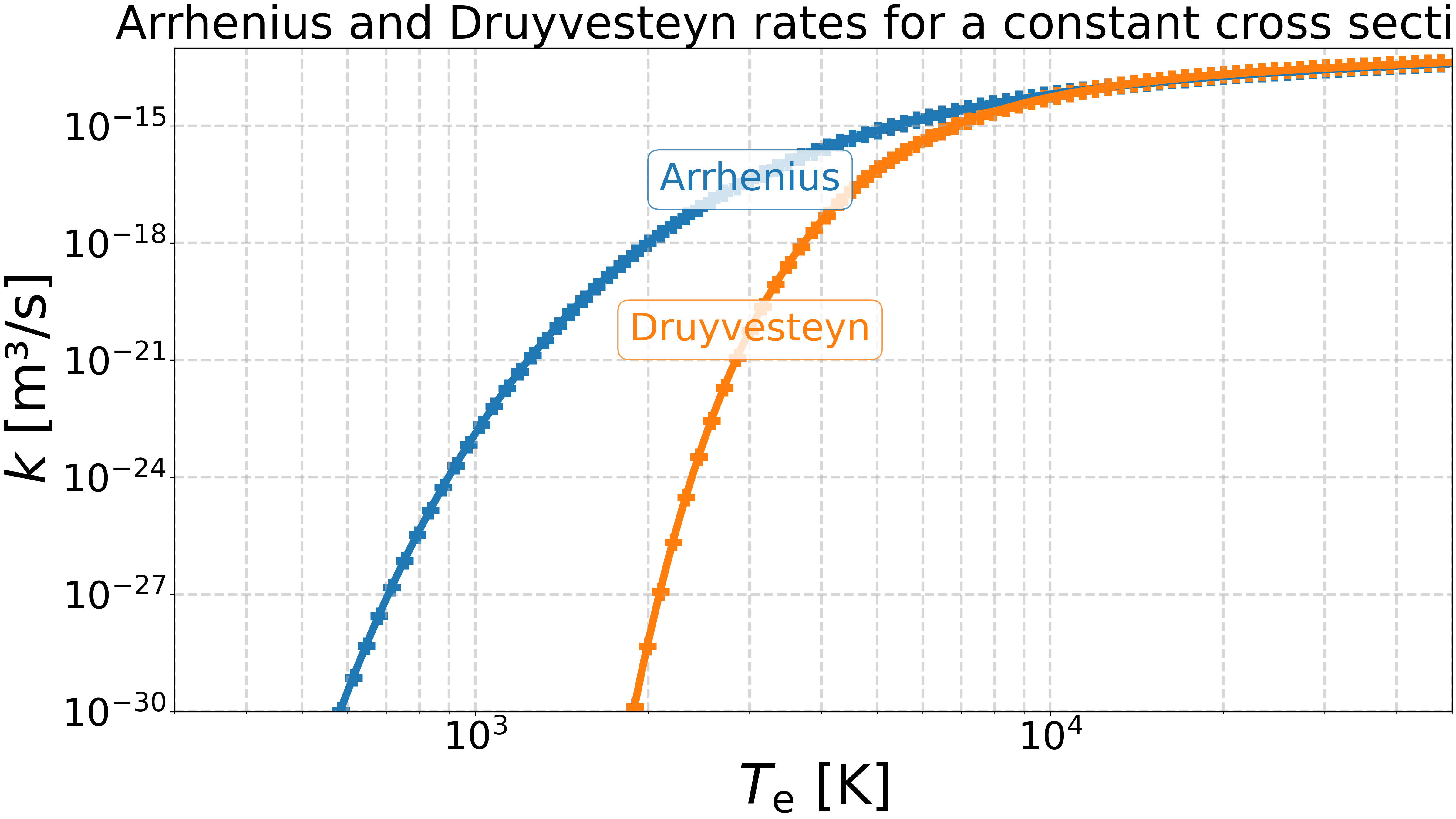
Plot the Arrhenius and Druyvesteyn rates.#
Also plot the expected reaction rate constant for a constant cross section.
fig, ax = plt.subplots()

for i, (computed_rate, expected_rate, text) in enumerate(
    [
        (arrhenius_rates_m3_per_s, arrhenius_rates_m3_per_s_expected, "Arrhenius"),
        (
            druyvesteyn_rates_m3_per_s,
            druyvesteyn_rates_m3_per_s_expected,
            "Druyvesteyn",
        ),
    ]
):
    ax.plot(electron_temperatures_K, computed_rate)
    color = ax.get_lines()[-1].get_color()
    ax.scatter(
        electron_temperatures_K[::10],
        expected_rate[::10],
        color=color,
        marker="+",
        s=200,
    )
    index = np.argmin(np.abs(electron_temperatures_K - 3_000))
    get_text(
        x=electron_temperatures_K[index],
        y=computed_rate[index],
        text=text,
        ax=ax,
        color=color,
    )

ax.set_xlabel(r"$T_\text{e}$ [K]")
ax.set_ylabel(r"$k$ [m³/s]")
ax.set_title("Arrhenius and Druyvesteyn rates for a constant cross section")
ax.set_xscale("log")
ax.set_yscale("log")
ax.set_xlim(300, 50000)
ax.set_ylim(1e-30, 1e-13)

plt.show()
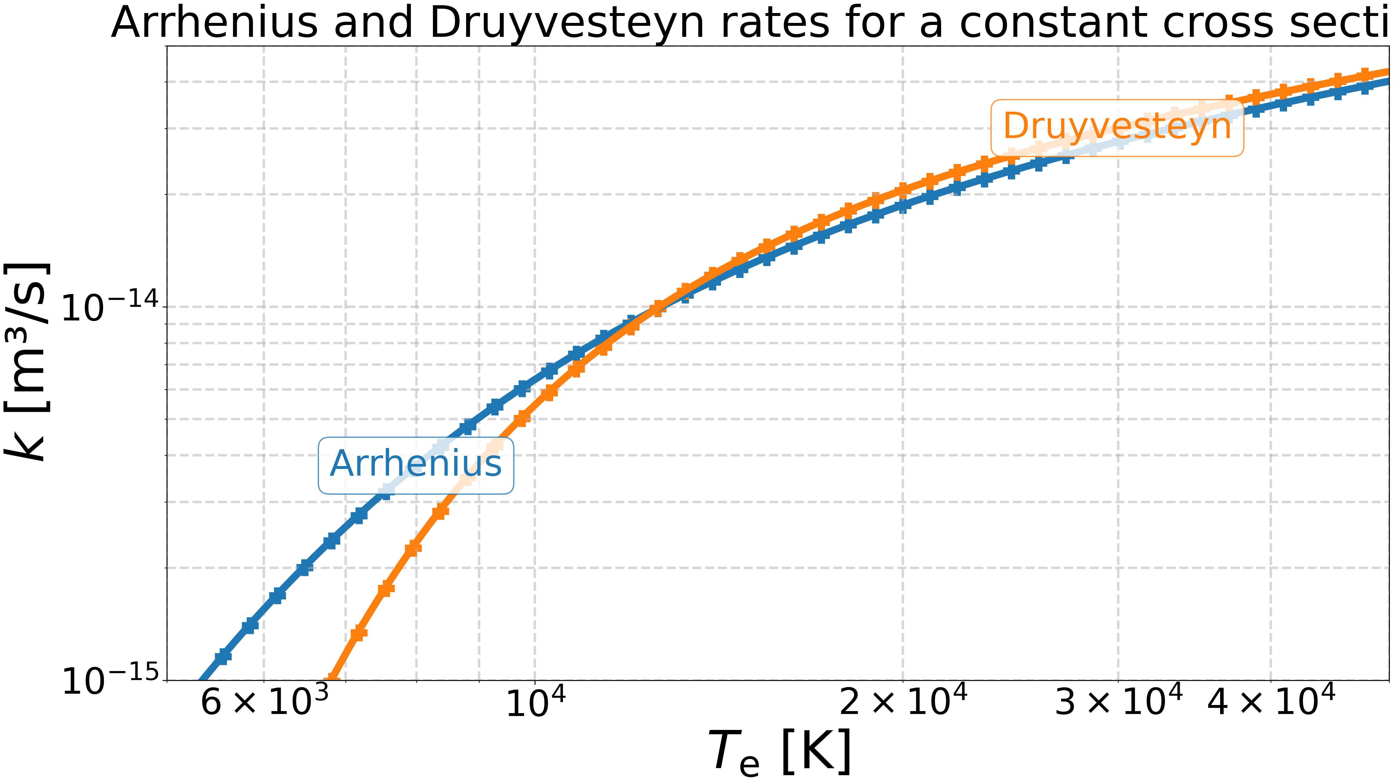
Same plot, zoomed in on the region of interest.
fig, ax = plt.subplots()

for i, (computed_rate, expected_rate, text, xlabel) in enumerate(
    [
        (
            arrhenius_rates_m3_per_s,
            arrhenius_rates_m3_per_s_expected,
            "Arrhenius",
            8000,
        ),
        (
            druyvesteyn_rates_m3_per_s,
            druyvesteyn_rates_m3_per_s_expected,
            "Druyvesteyn",
            3e4,
        ),
    ]
):
    ax.plot(electron_temperatures_K, computed_rate)
    color = ax.get_lines()[-1].get_color()
    ax.scatter(
        electron_temperatures_K[::10],
        expected_rate[::10],
        color=color,
        marker="+",
        s=200,
    )
    index = np.argmin(np.abs(electron_temperatures_K - xlabel))
    get_text(
        x=electron_temperatures_K[index],
        y=computed_rate[index],
        text=text,
        ax=ax,
        color=color,
    )

ax.set_xlabel(r"$T_\text{e}$ [K]")
ax.set_ylabel(r"$k$ [m³/s]")
ax.set_title("Arrhenius and Druyvesteyn rates for a constant cross section")
ax.set_xscale("log")
ax.set_yscale("log")
ax.set_xlim(5000, 50000)
ax.set_ylim(1e-15, 5e-14)

plt.show()
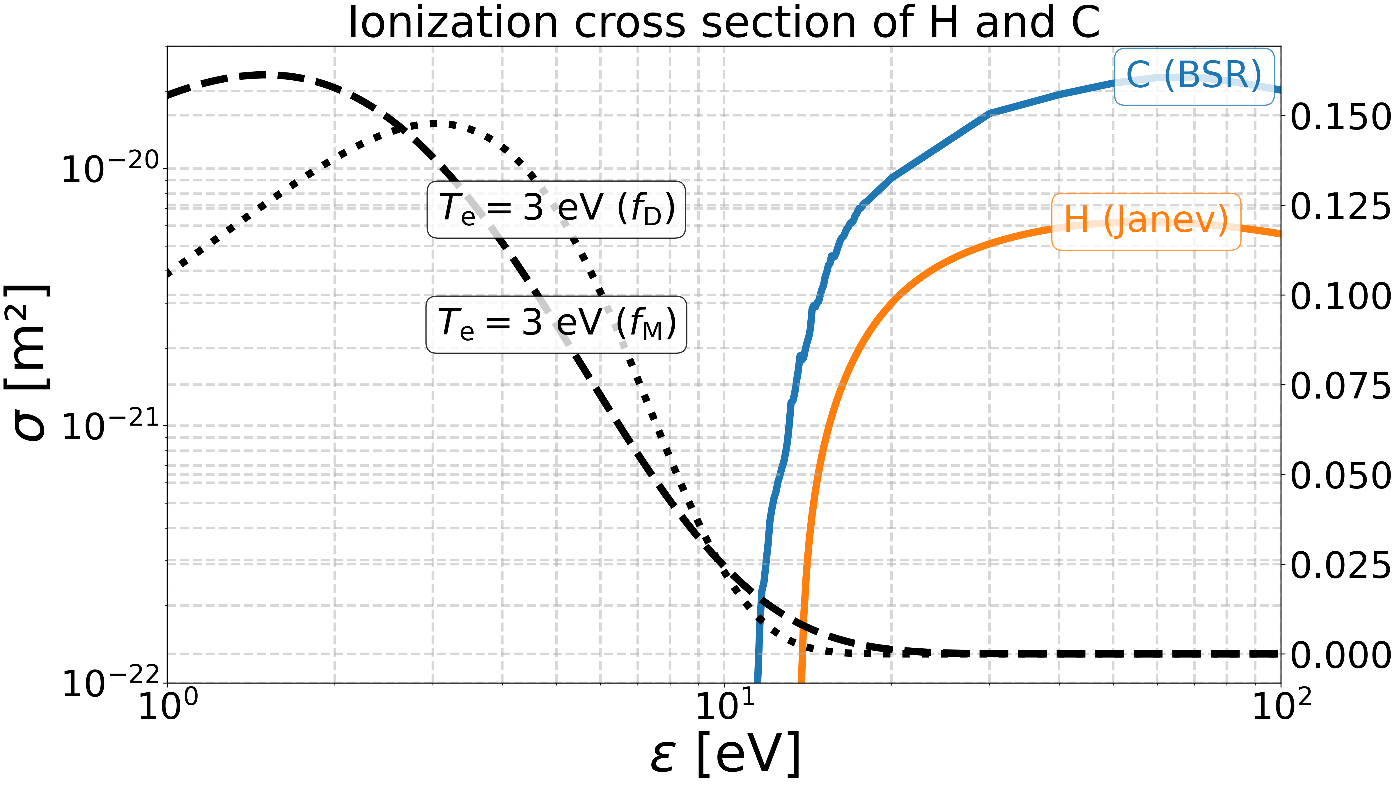
Also compute and plot the rates for the ionization cross section of H and C.#
lx = LXCat(verbose=False)

# Get the ionization cross section of C.
lx.read(file=get_path_to_data("kin", "cross_section", "C", "BSR.txt"))
ionization_cross_section_C_data = lx.species["C"].collisions["C -> C^+"]
ionization_cross_section_C_m2 = ionization_cross_section_C_data.cross_section_cm2 * 1e-4
energies_J_C = ionization_cross_section_C_data.energy_eV * u.eV_to_J

# Get the ionization cross section of H.
lx.read(
    file=get_path_to_data("kin", "cross_section", "H", "janev_cross_sections_H.txt")
)
ionization_cross_section_H_data = lx.species["H"].collisions["H -> H^+"]
ionization_cross_section_H_m2 = ionization_cross_section_H_data.cross_section_cm2 * 1e-4
energies_J_H = ionization_cross_section_H_data.energy_eV * u.eV_to_J

# Plot the ionization cross section of H and C.
fig, ax = plt.subplots()
ax.plot(ionization_cross_section_C_data.energy_eV, ionization_cross_section_C_m2)
get_text(
    x=ionization_cross_section_C_data.energy_eV[
        np.argmax(ionization_cross_section_C_m2)
    ],
    y=ionization_cross_section_C_m2[np.argmax(ionization_cross_section_C_m2)],
    text="C (BSR)",
    ax=ax,
)
color_C = ax.get_lines()[-1].get_color()
# radius_c_m = 137e-12 / 2  # Mean of atomic radius (70 pm and 67 pm)
# ax.hlines(
#     y=np.pi * radius_c_m**2,
#     xmin=1,
#     xmax=100,
#     color=color_C,
#     linestyle="--",
# )

ax.plot(ionization_cross_section_H_data.energy_eV, ionization_cross_section_H_m2)
get_text(
    x=ionization_cross_section_H_data.energy_eV[
        np.argmax(ionization_cross_section_H_m2)
    ],
    y=ionization_cross_section_H_m2[np.argmax(ionization_cross_section_H_m2)],
    text="H (Janev)",
    ax=ax,
)
color_H = ax.get_lines()[-1].get_color()
# radius_h_m = 39e-12  # Mean of atomic radius (25 pm and 53 pm)
# ax.hlines(
#     y=np.pi * radius_h_m**2,
#     xmin=1,
#     xmax=100,
#     color=color_H,
#     linestyle="--",
# )


# Plot the Maxwellian and Druyvesteyn distribution functions in energy.
T = 3 * u.eV_to_K  # K
energies = np.linspace(0, 100, 10000) * u.eV_to_J  # J
f_M = maxwellian_distribution_function_in_energy(T, energies)  # J^-1
f_D = druyvesteyn_distribution_function_in_energy(T, energies)  # J^-1

ax2 = ax.twinx()
x_text_in_eV = 5
ax2.plot(energies * u.J_to_eV, f_M / u.J_to_eV, color="black", linestyle="--")
ax2.plot(energies * u.J_to_eV, f_D / u.J_to_eV, color="black", linestyle=":")
y_text = f_M[np.argmin(np.abs(energies * u.J_to_eV - x_text_in_eV))] / u.J_to_eV
get_text(
    x_text_in_eV,
    y_text,
    rf"$T_\mathrm{{e}}={int(T * u.K_to_eV):,} \ \mathrm{{eV}}$ ($f_\text{{M}}$)",
    ax=ax2,
    color="black",
)
y_text = f_D[np.argmin(np.abs(energies * u.J_to_eV - x_text_in_eV))] / u.J_to_eV
get_text(
    x_text_in_eV,
    y_text,
    rf"$T_\mathrm{{e}}={int(T * u.K_to_eV):,} \ \mathrm{{eV}}$ ($f_\text{{D}}$)",
    ax=ax2,
    color="black",
)


ax.set_xlabel(r"$\varepsilon$ [eV]")
ax.set_ylabel(r"$\sigma$ [m²]")
ax.set_title("Ionization cross section of H and C")
ax.set_xscale("log")
ax.set_yscale("log")
ax.set_xlim(1, 100)
ax.set_ylim(1e-22, 3e-20)
plt.show()
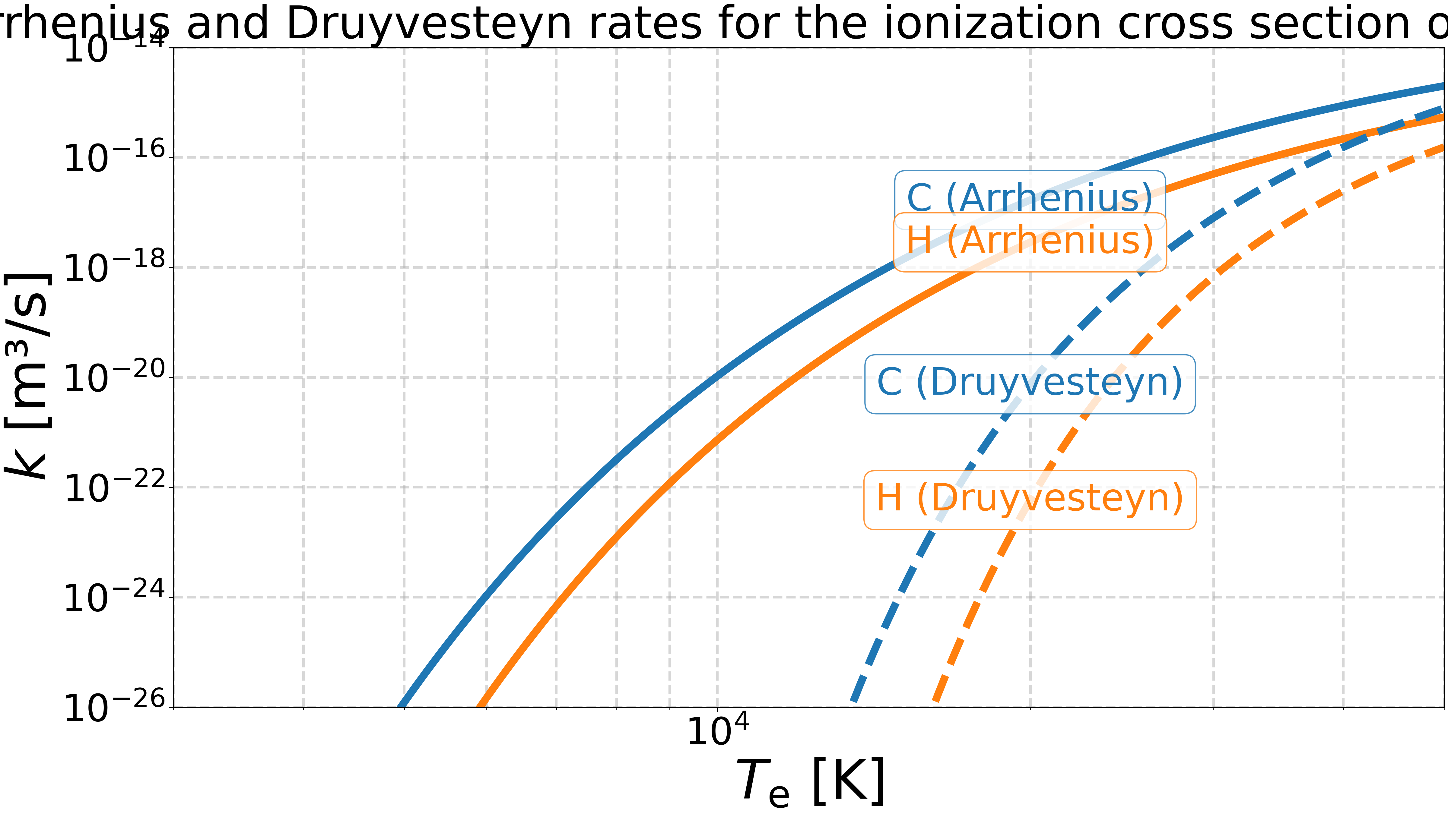
Compute the Arrhenius and Druyvesteyn rates for the ionization cross section of H and C.
arrhenius_rates_m3_per_s_C = np.zeros_like(electron_temperatures_K)
arrhenius_rates_m3_per_s_H = np.zeros_like(electron_temperatures_K)
druyvesteyn_rates_m3_per_s_C = np.zeros_like(electron_temperatures_K)
druyvesteyn_rates_m3_per_s_H = np.zeros_like(electron_temperatures_K)
for i, T in enumerate(electron_temperatures_K):
    arrhenius_rates_m3_per_s_C[i] = compute_electronic_reaction_rate_constant(
        T, ionization_cross_section_C_m2, energies_J_C
    )
    arrhenius_rates_m3_per_s_H[i] = compute_electronic_reaction_rate_constant(
        T, ionization_cross_section_H_m2, energies_J_H
    )
    druyvesteyn_rates_m3_per_s_C[i] = (
        compute_electronic_reaction_rate_constant_druyvesteyn(
            T, ionization_cross_section_C_m2, energies_J_C
        )
    )
    druyvesteyn_rates_m3_per_s_H[i] = (
        compute_electronic_reaction_rate_constant_druyvesteyn(
            T, ionization_cross_section_H_m2, energies_J_H
        )
    )

fig, ax = plt.subplots()
T_text = 20_000

ax.plot(electron_temperatures_K, arrhenius_rates_m3_per_s_C, color=color_C)
get_text(
    x=electron_temperatures_K[np.argmin(np.abs(electron_temperatures_K - T_text))],
    y=arrhenius_rates_m3_per_s_C[np.argmin(np.abs(electron_temperatures_K - T_text))],
    text="C (Arrhenius)",
    ax=ax,
)
ax.plot(electron_temperatures_K, arrhenius_rates_m3_per_s_H, color=color_H)
get_text(
    x=electron_temperatures_K[np.argmin(np.abs(electron_temperatures_K - T_text))],
    y=arrhenius_rates_m3_per_s_H[np.argmin(np.abs(electron_temperatures_K - T_text))],
    text="H (Arrhenius)",
    ax=ax,
)
ax.plot(electron_temperatures_K, druyvesteyn_rates_m3_per_s_C, color=color_C, ls="--")
get_text(
    x=electron_temperatures_K[np.argmin(np.abs(electron_temperatures_K - T_text))],
    y=druyvesteyn_rates_m3_per_s_C[np.argmin(np.abs(electron_temperatures_K - T_text))],
    text="C (Druyvesteyn)",
    ax=ax,
)
ax.plot(electron_temperatures_K, druyvesteyn_rates_m3_per_s_H, color=color_H, ls="--")
get_text(
    x=electron_temperatures_K[np.argmin(np.abs(electron_temperatures_K - T_text))],
    y=druyvesteyn_rates_m3_per_s_H[np.argmin(np.abs(electron_temperatures_K - T_text))],
    text="H (Druyvesteyn)",
    ax=ax,
)


ax.set_xlabel(r"$T_\text{e}$ [K]")
ax.set_ylabel(r"$k$ [m³/s]")
ax.set_title(
    "Arrhenius and Druyvesteyn rates for the ionization cross section of H and C"
)
ax.set_xscale("log")
ax.set_yscale("log")
ax.set_xlim(3000, 50000)
ax.set_ylim(1e-26, 1e-14)
plt.show()
Total running time of the script: (0 minutes 3.090 seconds)