
Note
Go to the end to download the full example code.
Tutorial 7 — Four circuits driving the same constant-mass discharge.#
What this shows: the same 0D2T constant-mass plasma reactor
(Isomass2TVolumeReactor, C++
backend), driven in turn by four different circuits, all through the same
electric_circuit.compute_plasma_voltage(t, R_p) call the reactor already makes –
demonstrating just how differently a discharge behaves depending on what limits the
current flowing into it.
Transmission line (see
TransmissionLineResistiveCircuit): the generator’s current is bounded by the cable’s characteristic impedance \(Z_c\) – the discharge stays in a strongly two-temperature regime (\(T_e \gg T_g\)).Direct voltage (no circuit element at all): the plasma sees the generator’s own voltage directly, unclamped. Nothing pulls the source voltage down as the plasma ionizes and its conductivity rises – unlike every circuit with an impedance in series, there is no negative feedback here, so the Joule heating runs away. Run until the solver itself fails.
`RC_Rp_Circuit` (see
RC_Rp_Circuit): a trapezoidal generator in series with a small parasitic resistance \(R_{par}=100\,\text{m}\Omega\), feeding a node where a \(C=10\,\text{pF}\) capacitor sits in parallel with the plasma resistance. \(R_{par}\) is small enough that it barely limits the current once the plasma is well-ionized (\(R_p \gg R_{par}\)) – weaker current limiting than the transmission line, but not zero like case 2 – so the discharge heats further than case 1, without literally diverging like case 2.`TransmissionLineRCLoadCircuit` (see
TransmissionLineRCLoadCircuit): the same transmission line as case 1, now terminated by a \(C=20\,\text{pF}\) capacitor in parallel with the plasma resistance – the cable’s \(Z_c\) still limits the current, but the capacitor also stores charge at the load node, smoothing the plasma voltage relative to the plain transmission line.
import cantera as ct
import matplotlib.pyplot as plt
import numpy as np

import rizer.kinetics.extensible_rate  # noqa: F401 (Register CH4 custom rates)
import rizer.misc.units as u
from rizer.electrical_model.circuit.adapter import DrivenCircuitAdapter
from rizer.electrical_model.circuit.rc_rp_circuit import RC_Rp_Circuit
from rizer.electrical_model.circuit.transmission_line_circuit import (
    TransmissionLineRCLoadCircuit,
    TransmissionLineResistiveCircuit,
)
from rizer.electrical_model.components.cable import IdealCable
from rizer.electrical_model.components.generator import TrapezoidalGenerator
from rizer.electrical_model.components.source_circuit import ResistiveSourceCircuit
from rizer.misc.plt_utils import set_mpl_style
from rizer.misc.utils import get_path_to_data
from rizer.models.nrp.isomass_2T_volume_reactor_cpp import Isomass2TVolumeReactor
from rizer.transport.loaders import (
    get_default_collision_frequency_model,
    get_momentum_transfer_collision_frequencies_list,
)

set_mpl_style()
Shared plasma/mechanism/geometry setup (mirrors plot_0d_cpp_vs_python.py), and
the same trapezoidal generator pulse driving all four circuits.
mechanism = str(get_path_to_data("mechanisms") / "Goutier2025" / "CH4_to_C2H2.yaml")
gap = 3.8e-3  # [m]
radius = 500e-6  # [m]
V0 = gap * np.pi * radius**2  # [m^3]

P0 = ct.one_atm
Tg_0 = 1000.0  # [K]
Te_0 = 1000.0  # [K]
ne_0 = 1.0e19  # [m^-3]
n_tot = P0 / (u.k_b * Tg_0)
x_e = ne_0 / n_tot

cfm = get_default_collision_frequency_model()

U_ON, T_RISE, T_ON, T_FALL, R_G = (
    7e3,
    5e-9,
    6e-9,
    6e-9,
    1.0,
)  # generator pulse [V, s, s, s, Ohm]
T_END = 100e-9  # [s]
DT_OUT = 1e-9  # [s]


def _make_plasma() -> ct.Solution:
    plasma = ct.Solution(mechanism, "plasma", transport_model=None)
    plasma.Te = Te_0
    plasma.TPX = Tg_0, P0, f"CH4:{1 - 2 * x_e:.6e}, e-:{x_e:.6e}, CH4+:{x_e:.6e}"
    return plasma


mtcf = get_momentum_transfer_collision_frequencies_list(
    _make_plasma().species_names, cfm
)


def _make_reactor(electric_circuit) -> Isomass2TVolumeReactor:
    plasma = _make_plasma()
    return Isomass2TVolumeReactor(
        plasma,
        mechanism,
        "plasma",
        mtcf,
        mass=plasma.density * V0,
        gap=gap,
        electric_circuit=electric_circuit,
        polytropic_index=np.inf,
        p_ext=P0,
    )


def _electron_density(reactor: Isomass2TVolumeReactor) -> float:
    """Mirrors `plot_0d_cpp_vs_python.py::reactor_electron_density`."""
    state = np.asarray(reactor.get_state())
    Tg, Te, V, Y = state[0], state[1], state[2], state[3:]
    rho = reactor.plasma_mass / V
    return reactor._r0d.electron_density(Tg, Te, np.ascontiguousarray(Y), rho)


def _run_case(
    reactor: Isomass2TVolumeReactor, net: ct.ReactorNet
) -> dict[str, np.ndarray]:
    """Advance `reactor` on the shared DT_OUT/T_END grid, collecting Tg/Te/ne/Vp.

    `net.max_time_step` must already be configured by the caller before this runs
    (case-specific: e.g. `window_span / 2` for an adapter-wrapped circuit).
    """
    t_hist, Tg_hist, Te_hist = [0.0], [Tg_0], [Te_0]
    ne_hist, Vp_hist = [ne_0], [0.0]  # Vp_0 matches the reactor's own initial 0.0.
    for t in np.arange(DT_OUT, T_END, DT_OUT):
        net.advance(t)
        state = np.asarray(reactor.get_state())
        t_hist.append(net.time)
        Tg_hist.append(state[0])
        Te_hist.append(state[1])
        ne_hist.append(_electron_density(reactor))
        Vp_hist.append(reactor.plasma_voltage)
    return {
        "t": np.array(t_hist),
        "Tg": np.array(Tg_hist),
        "Te": np.array(Te_hist),
        "ne": np.array(ne_hist),
        "Vp": np.array(Vp_hist),
    }
Case 1: transmission line – current bounded by the cable’s characteristic impedance Z_c.
line_circuit = TransmissionLineResistiveCircuit(
    source=ResistiveSourceCircuit(
        TrapezoidalGenerator(U_on=U_ON, t_rise=T_RISE, t_on=T_ON, t_fall=T_FALL),
        R_g=R_G,
    ),
    cable=IdealCable(L=6.2, Z_c=75.0, c=1.9e8),
    include_reflections=True,
)
reactor_line = _make_reactor(line_circuit)
net_line = ct.ReactorNet([reactor_line])
net_line.max_time_step = 1e-10

results_line = _run_case(reactor_line, net_line)
print(
    f"Case 1 (transmission line): completed, peak Te = {results_line['Te'].max():.0f} K"
)
Case 1 (transmission line): completed, peak Te = 37236 K
Case 2: direct voltage – no element between the generator and the plasma at all.
Deliberately unstable: nothing pulls the source voltage down as the plasma
ionizes, so Joule heating runs away. Run in an explicit net.step() loop
(rather than net.advance) with NO cap on net.max_time_step – letting
CVODE’s own adaptive step control hit the failure on its own terms, instead of
masking the divergence behind artificially small forced steps.
class _DirectVoltageLoad:
    """Example-local: the plasma sees the generator's own voltage, unclamped.

    Deliberately not a library class -- this is a one-line degenerate case (no
    current limiting at all), not a reusable circuit.
    """

    def __init__(self, generator: TrapezoidalGenerator) -> None:
        self.generator = generator

    def compute_plasma_voltage(self, t: float, R_p: float) -> float:
        """Return the generator's own voltage, ignoring `R_p` entirely."""
        return self.generator.generator_voltage(t)


direct_circuit = _DirectVoltageLoad(
    TrapezoidalGenerator(U_on=U_ON, t_rise=T_RISE, t_on=T_ON, t_fall=T_FALL)
)
reactor_direct = _make_reactor(direct_circuit)
net_direct = ct.ReactorNet([reactor_direct])

_t_direct = [0.0]
_Tg_direct, _Te_direct = [Tg_0], [Te_0]
_ne_direct, _Vp_direct = [ne_0], [0.0]
failure_reason = None
while net_direct.time < T_END:
    try:
        t_now = net_direct.step()
    except ct.CanteraError as exc:
        failure_reason = f"solver failure ({type(exc).__name__})"
        break
    state = np.asarray(reactor_direct.get_state())
    Tg_k, Te_k = state[0], state[1]
    if not (np.isfinite(Tg_k) and np.isfinite(Te_k)):
        failure_reason = "Tg/Te became non-finite"
        break
    _t_direct.append(t_now)
    _Tg_direct.append(Tg_k)
    _Te_direct.append(Te_k)
    _ne_direct.append(_electron_density(reactor_direct))
    _Vp_direct.append(reactor_direct.plasma_voltage)
results_direct = {
    "t": np.array(_t_direct),
    "Tg": np.array(_Tg_direct),
    "Te": np.array(_Te_direct),
    "ne": np.array(_ne_direct),
    "Vp": np.array(_Vp_direct),
}
print(
    f"Case 2 (direct voltage): {failure_reason or 'completed'} at "
    f"t = {results_direct['t'][-1] * 1e9:.3f} ns -- "
    f"last valid Te = {results_direct['Te'][-1]:.0f} K, "
    f"Tg = {results_direct['Tg'][-1]:.0f} K"
)
Case 2 (direct voltage): solver failure (CanteraError) at t = 7.275 ns -- last valid Te = 344770 K, Tg = 156582 K
Case 3: trapezoidal generator, small parasitic series resistance R_par, feeding a node where C is in parallel with R_p. Externally-driven mode only, so it is wrapped in a DrivenCircuitAdapter to answer the same compute_plasma_voltage(t, R_p) call the reactor already makes to TransmissionLineResistiveCircuit. window_span/net.max_time_step are tuned small (the circuit’s own RC time constant tau = C*(R_par || R_p) is of order 1 ps here) so the adapter re-syncs to the reactor’s rapidly-evolving R_p often enough.
R_PAR, C_PARASITIC = 0.1, 10e-12  # [Ohm], [F]
WINDOW_SPAN = 2e-11  # [s]

rc_generator = TrapezoidalGenerator(U_on=U_ON, t_rise=T_RISE, t_on=T_ON, t_fall=T_FALL)
rc_circuit = RC_Rp_Circuit(
    R_par=R_PAR, C=C_PARASITIC, u_mes=rc_generator.generator_voltage
)
rc_adapter = DrivenCircuitAdapter(
    rc_circuit,
    output=lambda t, y, R_p: rc_circuit.compute_plasma_voltage(t, y[0], R_p),
    window_span=WINDOW_SPAN,
    r_p_rtol=1e-2,
)
reactor_rc = _make_reactor(rc_adapter)
net_rc = ct.ReactorNet([reactor_rc])
net_rc.max_time_step = WINDOW_SPAN / 2

results_rc = _run_case(reactor_rc, net_rc)
print(f"Case 3 (RC_Rp_Circuit): completed, peak Te = {results_rc['Te'].max():.0f} K")
Case 3 (RC_Rp_Circuit): completed, peak Te = 84092 K
Case 4: the same cable/generator as case 1, now terminated by a capacitor in parallel with R_p (TransmissionLineRCLoadCircuit). Stateful, but – like TransmissionLineResistiveCircuit – called directly by the reactor: TransmissionLineRCLoadCircuit wraps its own internal DrivenCircuitAdapter, so no external adapter is needed here (unlike case 3). window_span is capped by the cable’s round trip (2*6.2/1.9e8 ~= 65 ns), and chosen well below it for causality margin; net.max_time_step follows the same window_span/2 pattern as case 3.
C_LOAD = 20e-12  # [F]
WINDOW_SPAN_LOAD = 1e-10  # [s]

line_c_circuit = TransmissionLineRCLoadCircuit(
    source=ResistiveSourceCircuit(
        TrapezoidalGenerator(U_on=U_ON, t_rise=T_RISE, t_on=T_ON, t_fall=T_FALL),
        R_g=R_G,
    ),
    cable=IdealCable(L=6.2, Z_c=75.0, c=1.9e8),
    C=C_LOAD,
    window_span=WINDOW_SPAN_LOAD,
    include_reflections=True,
)
reactor_line_c = _make_reactor(line_c_circuit)
net_line_c = ct.ReactorNet([reactor_line_c])
net_line_c.max_time_step = WINDOW_SPAN_LOAD / 2

results_line_c = _run_case(reactor_line_c, net_line_c)
print(
    "Case 4 (transmission line + C||Rp): completed, "
    f"peak Te = {results_line_c['Te'].max():.0f} K"
)
Case 4 (transmission line + C||Rp): completed, peak Te = 40355 K
Compare all four cases across Te, Tg, ne, and Vp.
CASES = [
    ("transmission line", results_line),
    # ("direct voltage", results_direct),
    # ("RC_Rp_Circuit", results_rc),
    ("transmission line + C||Rp", results_line_c),
]


def _compare_plot(key: str, y_label: str, title: str, log: bool = False) -> None:
    fig, ax = plt.subplots(figsize=(7, 4.5))
    for label, results in CASES:
        ax.plot(results["t"] * 1e9, results[key], label=label)
    ax.set_xlabel("t [ns]")
    ax.set_ylabel(y_label)
    ax.set_title(title)
    if log:
        ax.set_yscale("log")
    ax.legend(fontsize=9)
    ax.grid(alpha=0.3, which="both" if log else "major")
    plt.show()


_compare_plot("Te", r"$T_e$ [K]", "Electron temperature")
_compare_plot("Tg", r"$T_g$ [K]", "Gas temperature")
_compare_plot("ne", r"$n_e$ [m$^{-3}$]", "Electron density", log=True)
_compare_plot("Vp", r"$V_p$ [V]", "Plasma voltage")
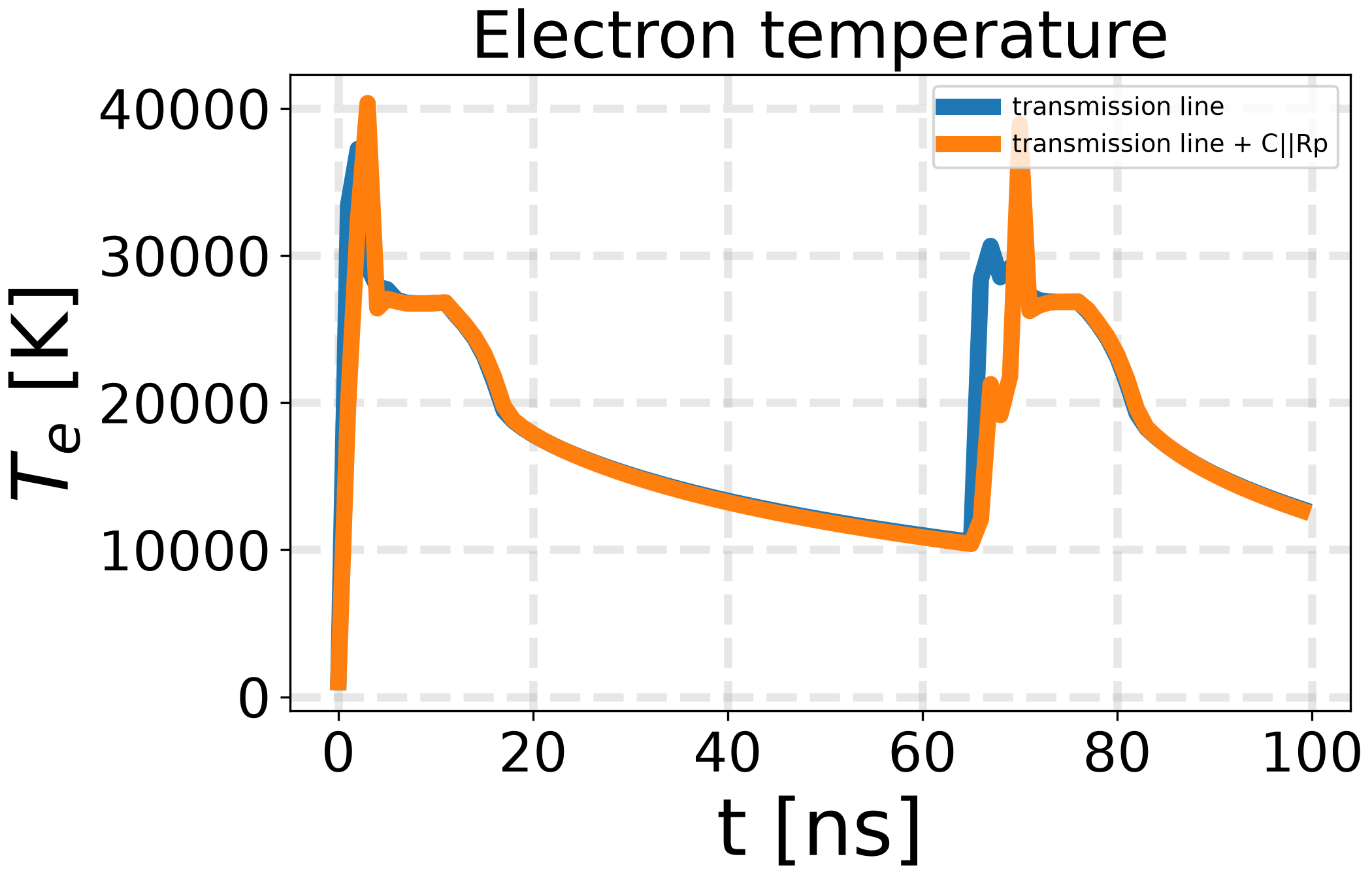
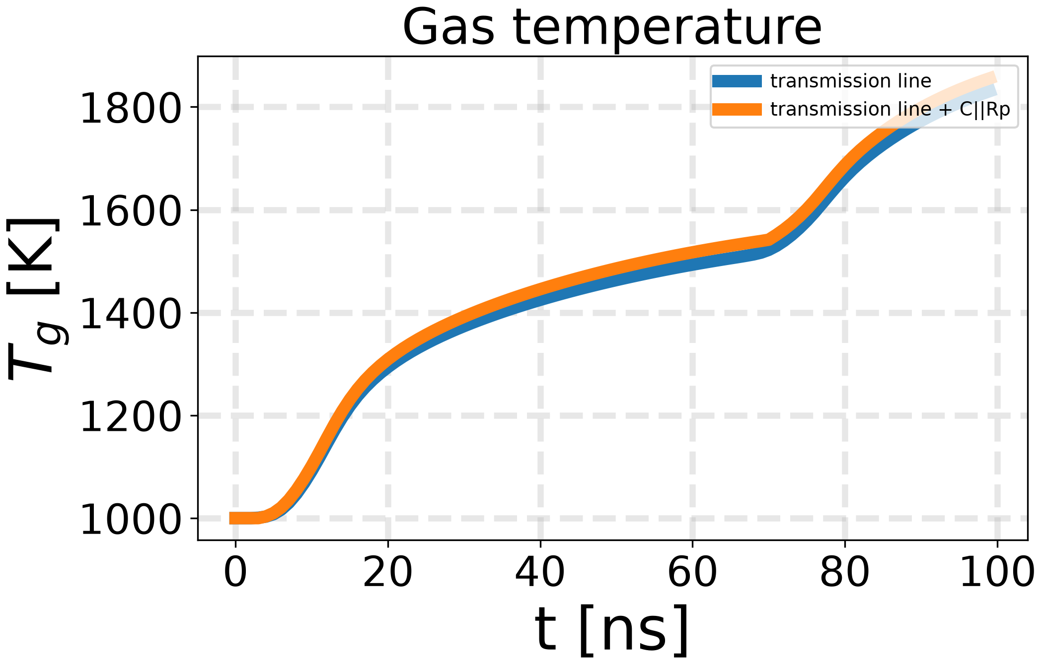
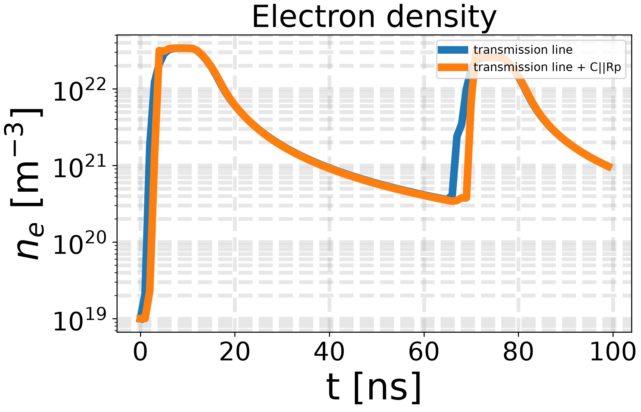
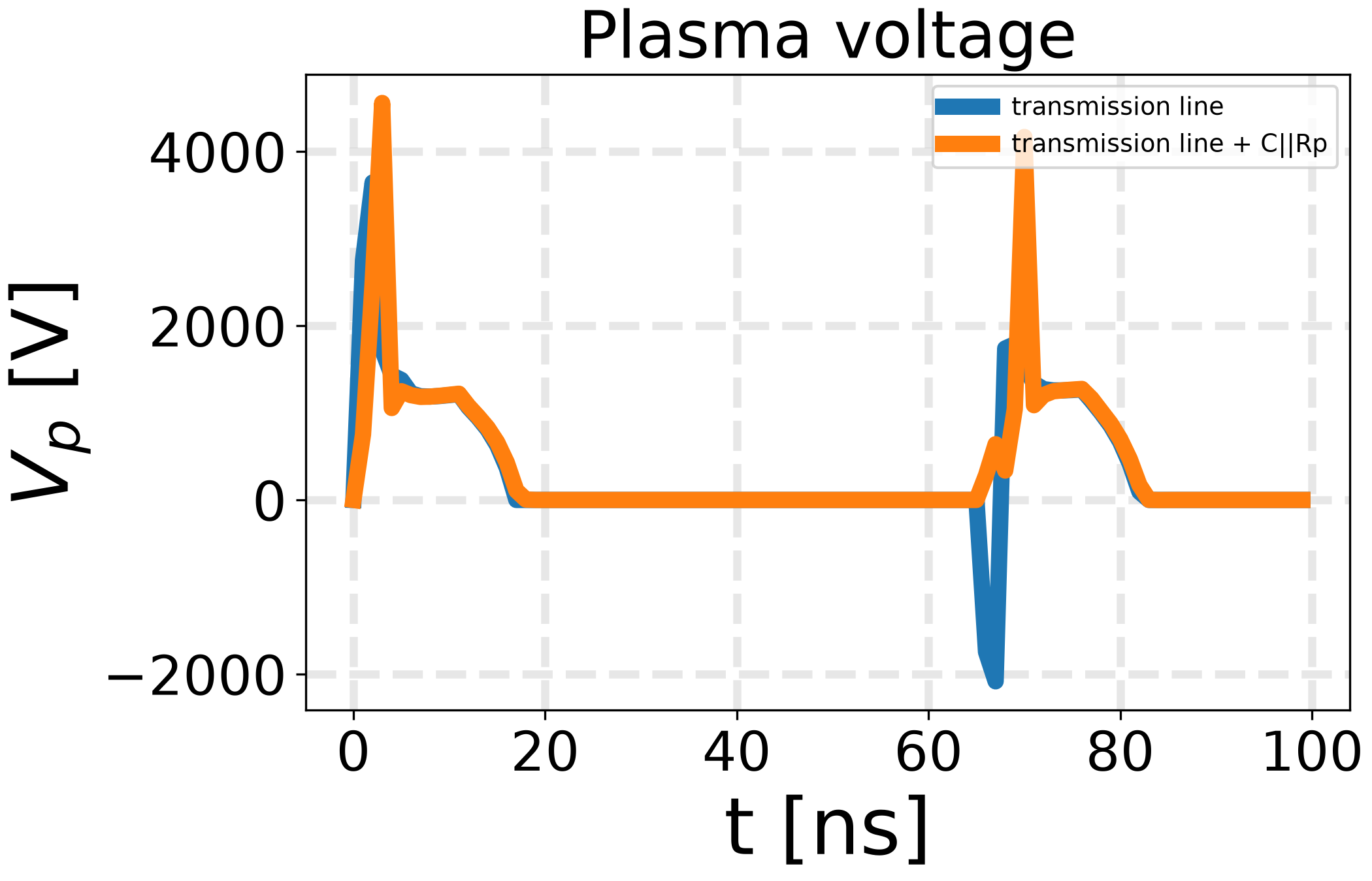
The transmission line keeps the discharge strongly two-temperature (\(T_e \gg T_g\)), bounded by \(Z_c\). The direct-voltage case has no negative feedback at all: current draw is unclamped as the plasma ionizes, and the solver itself fails a few nanoseconds in. The RC_Rp_Circuit sits closer to that runaway limit – \(R_{par}\) is small enough to barely limit the current once the plasma is well-ionized (\(R_p \gg R_{par}\)), so the discharge heats further than the transmission line and drives \(T_g\) toward \(T_e\) (full thermalization), without literally diverging like case 2. TransmissionLineRCLoadCircuit (case 4) tracks the plain transmission line closely – same \(Z_c\) current limiting – but the parallel capacitor smooths the plasma voltage V_p, and with it n_e, relative to the memoryless case 1.
Total running time of the script: (0 minutes 54.479 seconds)