Plot electron-impact cross sections for atomic carbon and rank its reactions.

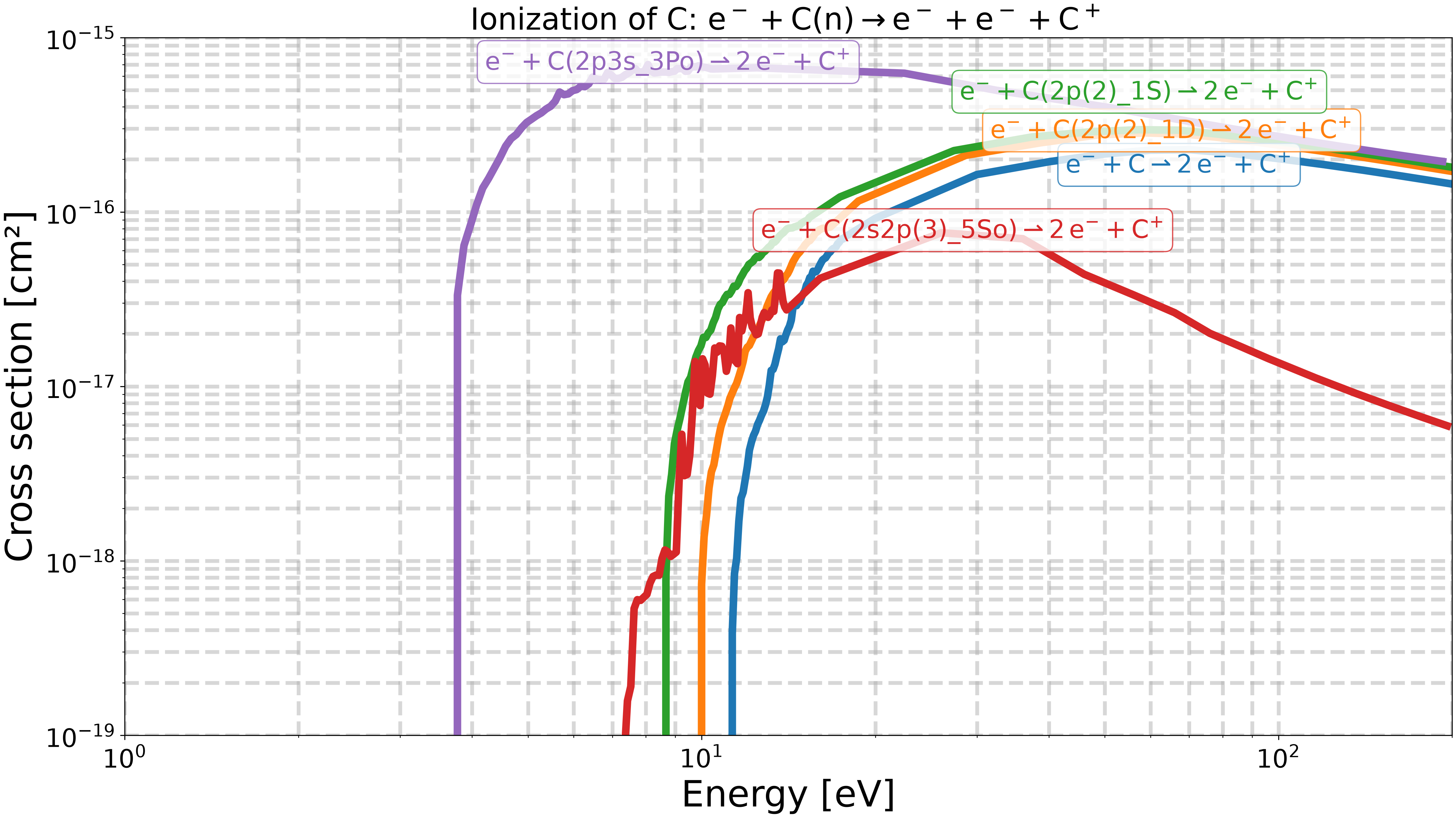
This example loads cross section data (BSR database) for the 5 electronic states of atomic carbon currently in the mechanism – ground (C), and the 4 excited states C(2p(2)_1D), C(2p(2)_1S), C(2s2p(3)_5So), C(2p3s_3Po) – and plots them in three groups:

• Excitation from the ground state (C): 4 reactions to the 4 excited states.

• Excitation between excited states: the 3 states below C(2p3s_3Po) each have a measured transition up to it (1D, 1S, 5So -> 3Po); no cross section exists yet for any other pair.

• Ionization to C⁺: from the ground state and each of the 4 excited states.

It then fits a Maxwellian reaction rate constant (rizer.kinetics.fit.fit_arrhenius.arrhenius_rate_fit_from_cross_section()) to each of the 13 reactions – the same assumption used to build the mechanism’s own forward reactions in scripts/mechanisms/build_electron_heavy_forward_reactions.py – and plots the 5 with the largest rate constant at \(T_e=4\) eV, a representative electron temperature for this discharge.

Data: data/cross_sections/lxcat_cross_sections/{C,C(2p(2)_1D),C(2p(2)_1S), C(2s2p(3)_5So),C(2p3s_3Po)}/BSR.txt, registered in data/cross_sections/lxcat_cross_sections/cross_sections_summary.yaml.

Tags: kinetics cross section reaction rate constant carbon

Import the required libraries.

import matplotlib.pyplot as plt
import numpy as np
from adjustText import adjust_text
from matplotlib.axes import Axes

import rizer.misc.units as u
from rizer.io.cross_sections.load_cross_sections import (
    CrossSectionData,
    filter_cross_sections_to_load,
    load_cross_sections_data,
    load_cross_sections_summary_yaml,
)
from rizer.kinetics.fit.fit_arrhenius import (
    ArrheniusRate,
    arrhenius_rate,
    arrhenius_rate_fit_from_cross_section,
)
from rizer.misc.plt_utils import (
    get_reaction_in_latex,
    get_text,
    set_mpl_style,
)

set_mpl_style(nb_columns=2)

# Representative electron temperature used to rank reactions by Maxwellian rate constant below.
T_E_REPRESENTATIVE = 4 * u.eV_to_K  # K

# How many of the 13 reactions to plot in the ranking figure.
TOP_N = 5

Load the carbon cross sections.

CARBON_SPECIES = [
    "C",
    "C(2p(2)_1D)",
    "C(2p(2)_1S)",
    "C(2s2p(3)_5So)",
    "C(2p3s_3Po)",
]

cross_sections: list[CrossSectionData] = load_cross_sections_data(
    filter_cross_sections_to_load(
        load_cross_sections_summary_yaml(), species_to_keep=CARBON_SPECIES
    )
)

GROUND_EXCITATION_EQUATIONS = {
    "e- + C => e- + C(2p(2)_1D)",
    "e- + C => e- + C(2p(2)_1S)",
    "e- + C => e- + C(2s2p(3)_5So)",
    "e- + C => e- + C(2p3s_3Po)",
}
EXCITED_EXCITATION_EQUATIONS = {
    "e- + C(2p(2)_1D) => e- + C(2p(2)_1S)",
    "e- + C(2p(2)_1D) => e- + C(2p3s_3Po)",
    "e- + C(2p(2)_1S) => e- + C(2p3s_3Po)",
    "e- + C(2s2p(3)_5So) => e- + C(2p3s_3Po)",
}
IONIZATION_EQUATIONS = {
    "e- + C => e- + e- + C+",
    "e- + C(2p(2)_1D) => e- + e- + C+",
    "e- + C(2p(2)_1S) => e- + e- + C+",
    "e- + C(2s2p(3)_5So) => e- + e- + C+",
    "e- + C(2p3s_3Po) => e- + e- + C+",
}

Helpers to plot cross sections.

def style_cross_section_axes(
    ax: Axes, title: str, xlim: tuple[float, float], ylim: tuple[float, float]
) -> None:
    """Apply common log-log styling for cross section plots."""
    ax.set_xlabel("Energy [eV]")
    ax.set_ylabel("Cross section [cm²]")
    ax.set_title(title)
    ax.set_xscale("log")
    ax.set_yscale("log")
    ax.set_xlim(left=xlim[0], right=xlim[1])
    ax.set_ylim(bottom=ylim[0], top=ylim[1])


def plot_cross_section_group(ax: Axes, group: list[CrossSectionData]) -> None:
    """Plot each cross section in `group`, with a label at its curve maximum."""
    texts = []
    for cross_section in group:
        energy_eV = cross_section.df.energy_eV
        cross_section_cm2 = cross_section.df.cross_section_cm2

        (line,) = ax.plot(energy_eV, cross_section_cm2)
        color = line.get_color()
        idx_max = np.argmax(cross_section_cm2)
        texts.append(
            get_text(
                float(energy_eV[idx_max]),
                float(cross_section_cm2[idx_max]),
                get_reaction_in_latex(cross_section.equation),
                ax=ax,
                color=color,
            )
        )
    adjust_text(texts, avoid_self=False)

Figure 1 – Excitation from the ground state.

ground_excitation = [
    cs for cs in cross_sections if cs.equation in GROUND_EXCITATION_EQUATIONS
]

fig1, ax1 = plt.subplots()
style_cross_section_axes(
    ax1,
    r"Electronic excitation of $\mathrm{C}$ from the ground state",
    xlim=(1, 3e2),
    ylim=(1e-19, 1e-15),
)
plot_cross_section_group(ax1, ground_excitation)
plt.show()

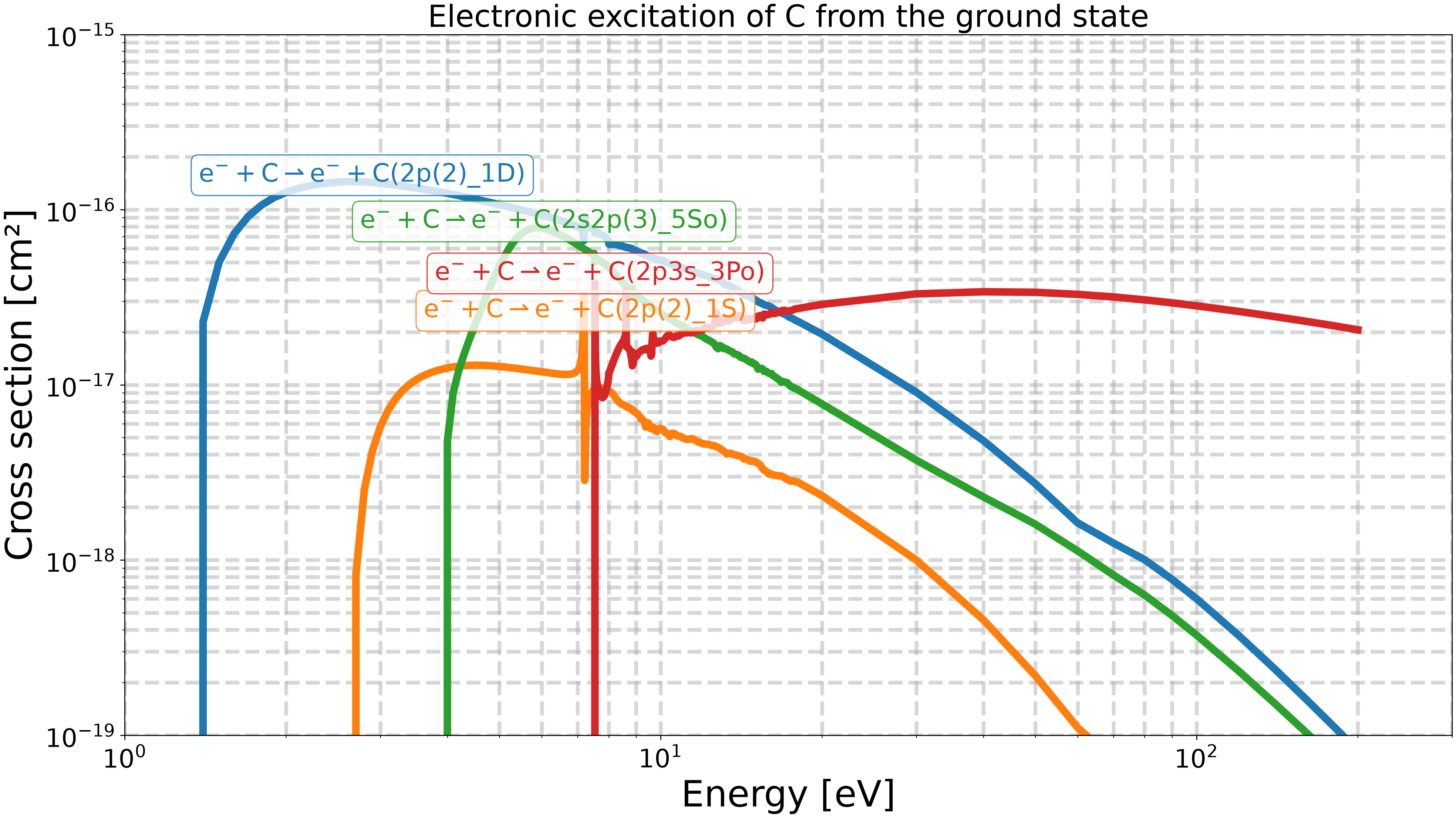
Figure 2 – Excitation between excited states.

excited_excitation = [
    cs for cs in cross_sections if cs.equation in EXCITED_EXCITATION_EQUATIONS
]

fig2, ax2 = plt.subplots()
style_cross_section_axes(
    ax2,
    r"Electronic excitation of $\mathrm{C}$ between excited states",
    xlim=(1, 3e2),
    ylim=(1e-19, 1e-15),
)
plot_cross_section_group(ax2, excited_excitation)
plt.show()

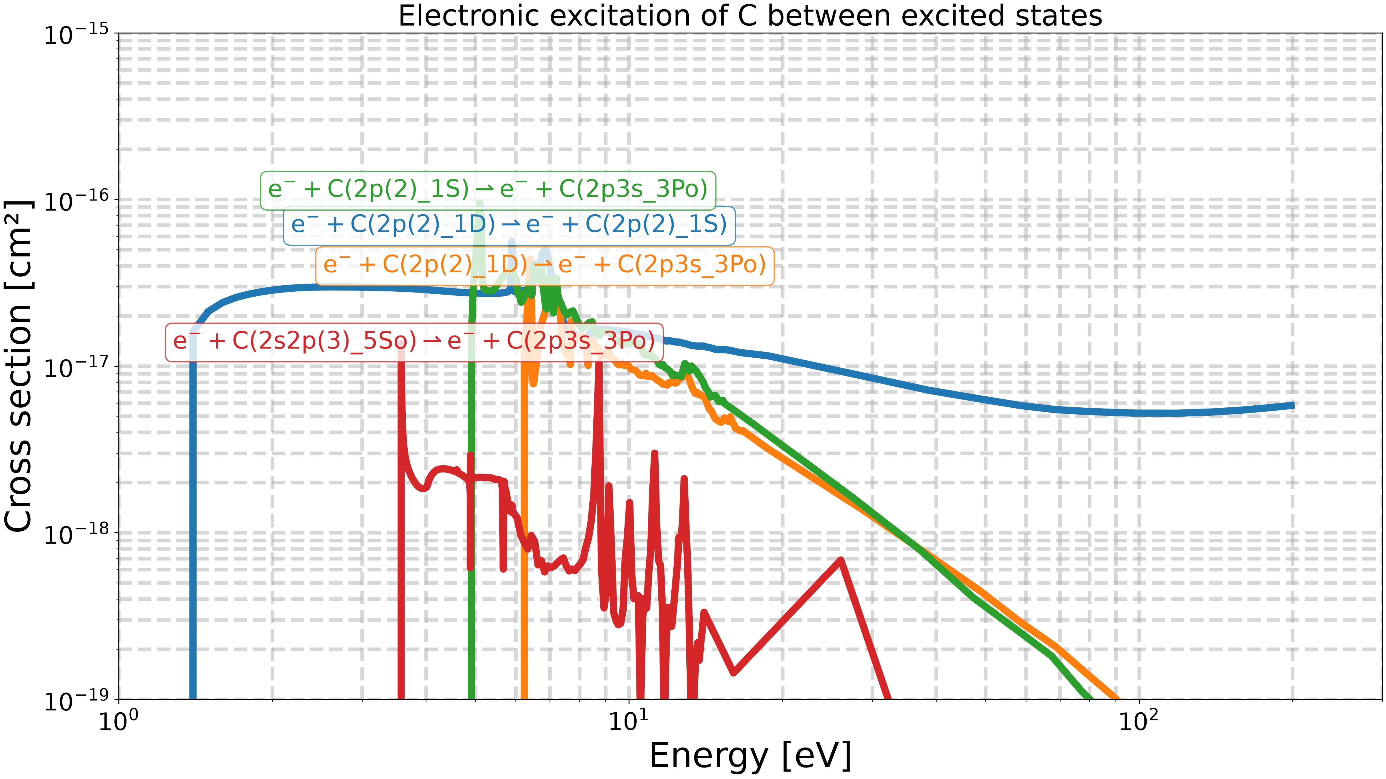
Figure 3 – Ionization to C⁺.

ionization = [cs for cs in cross_sections if cs.equation in IONIZATION_EQUATIONS]

fig3, ax3 = plt.subplots()
style_cross_section_axes(
    ax3,
    r"Ionization of $\mathrm{C}$: $\mathrm{e^- + C(n) \rightarrow e^- + e^- + C^+}$",
    xlim=(1, 2e2),
    ylim=(1e-19, 1e-15),
)
plot_cross_section_group(ax3, ionization)
plt.show()

Fit Maxwellian reaction rates and rank the top reactions.

Each of the 13 cross sections is fit once, over the same electron-temperature range used to build the mechanism’s own forward reactions, then ranked by rate constant at \(T_e=4\) eV – which reaction dominates is temperature-dependent (a low-threshold excitation wins at low \(T_e\); high-threshold ionization catches up at high \(T_e\)), so this ranking is a snapshot at one representative condition, not universal.

temperature_min = 1000  # [K]
temperature_max = 50_000  # [K]
nb_points_electron_temperatures = 1000  # [-]
electron_temperatures = np.geomspace(
    temperature_min, temperature_max, nb_points_electron_temperatures, dtype=float
)

rates: list[ArrheniusRate] = [
    arrhenius_rate_fit_from_cross_section(cross_section, electron_temperatures)
    for cross_section in cross_sections
]

k_at_T_representative = [
    arrhenius_rate(rate.A_m3_per_s, rate.b, rate.Ea_K, T_E_REPRESENTATIVE)
    for rate in rates
]
top_indices = np.argsort(k_at_T_representative)[::-1][:TOP_N]
top_rates = [rates[i] for i in top_indices]

print(f"Top {TOP_N} reactions by Maxwellian rate constant at T_e=4 eV:")
for rate, k in zip(top_rates, np.array(k_at_T_representative)[top_indices]):
    print(f"  {rate.equation}: k = {k:.2e} m3/s")

fig4, ax4 = plt.subplots()
texts = []
for rate in top_rates:
    k_fit = arrhenius_rate(rate.A_m3_per_s, rate.b, rate.Ea_K, electron_temperatures)
    (line,) = ax4.plot(electron_temperatures, k_fit)
    color = line.get_color()
    k_representative = arrhenius_rate(
        rate.A_m3_per_s, rate.b, rate.Ea_K, T_E_REPRESENTATIVE
    )
    ax4.scatter(
        [T_E_REPRESENTATIVE], [k_representative], color=color, marker="x", s=100
    )
    texts.append(
        get_text(
            T_E_REPRESENTATIVE,
            k_representative,
            get_reaction_in_latex(rate.equation),
            ax=ax4,
            color=color,
        )
    )
ax4.set_xlabel("Electron temperature [K]")
ax4.set_ylabel("Reaction rate constant [m³/s]")
ax4.set_title(f"Top {TOP_N} carbon reactions by Maxwellian rate at " r"$T_e=4$ eV")
ax4.set_xscale("log")
ax4.set_yscale("log")
ax4.set_ylim(bottom=1e-18, top=1e-13)
ax4.set_xlim(left=temperature_min, right=temperature_max)
adjust_text(texts, arrowprops=dict(arrowstyle="->", color="k"))
plt.show()

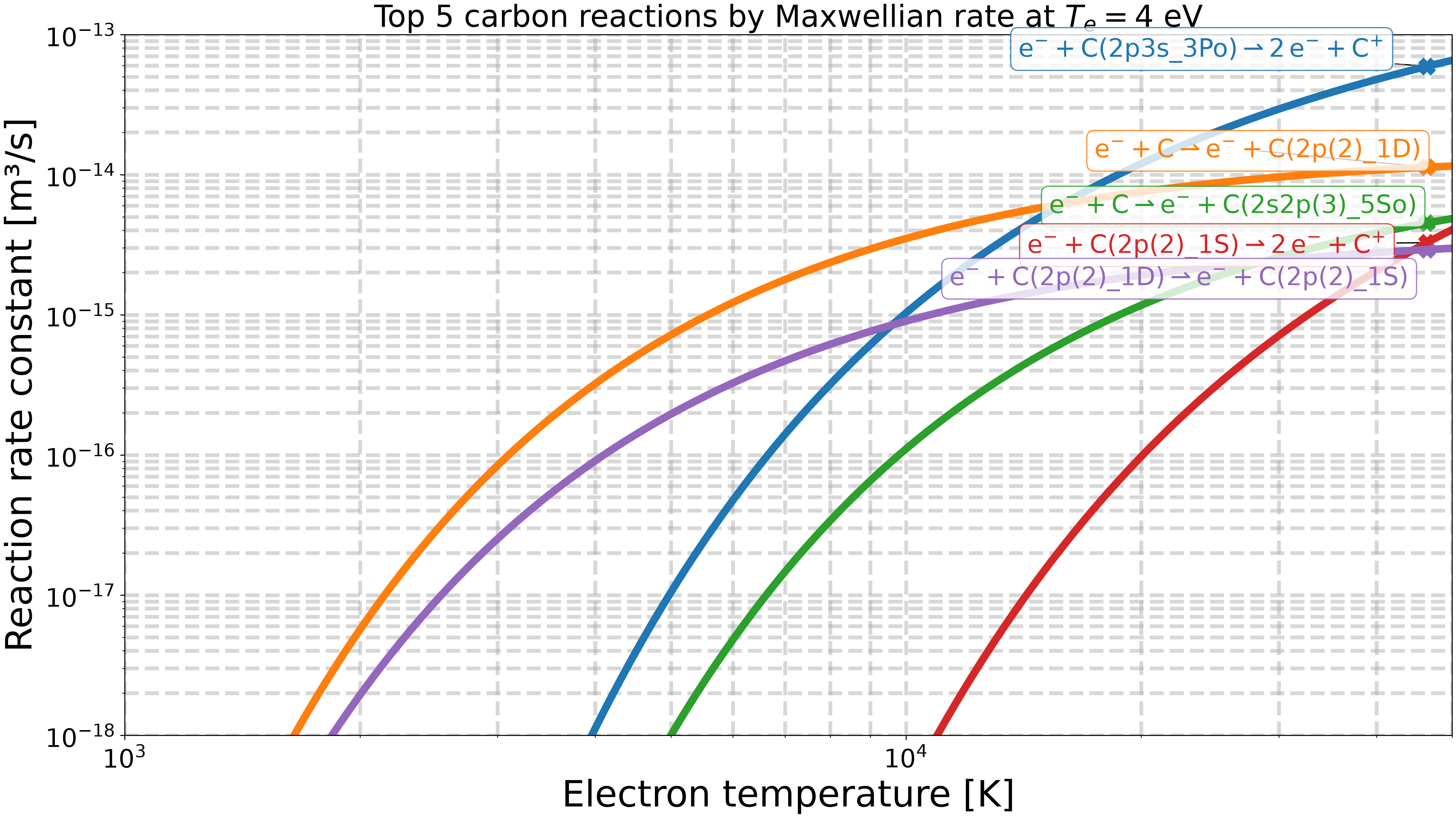
Top 5 reactions by Maxwellian rate constant at T_e=4 eV:
  e- + C(2p3s_3Po) => e- + e- + C+: k = 5.92e-14 m3/s
  e- + C => e- + C(2p(2)_1D): k = 1.13e-14 m3/s
  e- + C => e- + C(2s2p(3)_5So): k = 4.51e-15 m3/s
  e- + C(2p(2)_1S) => e- + e- + C+: k = 3.27e-15 m3/s
  e- + C(2p(2)_1D) => e- + C(2p(2)_1S): k = 2.92e-15 m3/s