
Note
Go to the end to download the full example code.
Tutorial 8 — Capacitive source networks: c_shunt vs c_parallel.#
What this shows: the same 0D2T constant-mass plasma reactor
(Isomass2TVolumeReactor, C++
backend), generator, and transmission line as Tutorial 7’s case 1
(TransmissionLineResistiveCircuit),
now driven in turn by three different source-side networks – comparing the
plain resistive source against a capacitor \(C_s\) placed at two different
positions relative to the source resistance \(R_g\).
Resistive source (see
ResistiveSourceCircuit): the baseline, identical to Tutorial 7’s case 1.`c_shunt` (see
CapacitiveSourceCircuit, drivingTransmissionLineCapacitiveSourceResistiveLoadCircuit): \(C_s\) shunts the source’s own output node to ground, in parallel with the cable’s input.`c_parallel` (see
ParallelCapacitiveSourceCircuit, drivingTransmissionLineParallelCapacitiveSourceResistiveLoadCircuit): the same \(C_s\) value instead bridges \(R_g\) itself, rather than shunting the output node.
Cases 2 and 3 use the same \(C_s\) – the point is that the two placements are
genuinely different networks (different ODEs, see
rizer.electrical_model’s README “Sources” section), not a parameter sweep of
one topology. Their governing equations also drive the capacitor differently in
strength: c_shunt’s forcing term is \(V_g/R_g\), c_parallel’s is
\(V_g/Z_c\) – with \(Z_c \gg R_g\) here, the same \(C_s\) perturbs the
plasma voltage far less for c_parallel than for c_shunt, shown below on its own
scale.
import cantera as ct
import matplotlib.pyplot as plt
import numpy as np

import rizer.kinetics.extensible_rate  # noqa: F401 (Register CH4 custom rates)
import rizer.misc.units as u
from rizer.electrical_model.circuit.transmission_line_circuit import (
    TransmissionLineCapacitiveSourceResistiveLoadCircuit,
    TransmissionLineParallelCapacitiveSourceResistiveLoadCircuit,
    TransmissionLineResistiveCircuit,
)
from rizer.electrical_model.components.cable import IdealCable
from rizer.electrical_model.components.generator import TrapezoidalGenerator
from rizer.electrical_model.components.source_circuit import (
    CapacitiveSourceCircuit,
    ParallelCapacitiveSourceCircuit,
    ResistiveSourceCircuit,
)
from rizer.misc.plt_utils import set_mpl_style
from rizer.misc.utils import get_path_to_data
from rizer.models.nrp.isomass_2T_volume_reactor_cpp import Isomass2TVolumeReactor
from rizer.transport.loaders import (
    get_default_collision_frequency_model,
    get_momentum_transfer_collision_frequencies_list,
)

set_mpl_style()
Shared plasma/mechanism/geometry setup (mirrors
plot_07_constant_mass_discharge_circuit_comparison.py), and the same
trapezoidal generator pulse driving all three source networks.
mechanism = str(get_path_to_data("mechanisms") / "Goutier2025" / "CH4_to_C2H2.yaml")
gap = 3.8e-3  # [m]
radius = 500e-6  # [m]
V0 = gap * np.pi * radius**2  # [m^3]

P0 = ct.one_atm
Tg_0 = 1000.0  # [K]
Te_0 = 1000.0  # [K]
ne_0 = 1.0e19  # [m^-3]
n_tot = P0 / (u.k_b * Tg_0)
x_e = ne_0 / n_tot

cfm = get_default_collision_frequency_model()

U_ON, T_RISE, T_ON, T_FALL, R_G = (
    7e3,
    5e-9,
    6e-9,
    6e-9,
    1.0,
)  # generator pulse [V, s, s, s, Ohm]
T_END = 100e-9  # [s]
DT_OUT = 1e-9  # [s]

CABLE = IdealCable(L=6.2, Z_c=75.0, c=1.9e8)  # round_trip_time = 2*6.2/1.9e8 ~= 65.3 ns
C_S = 20e-12  # [F], shared by both capacitive-source cases -- see module docstring
WINDOW_SPAN = 1e-9  # [s], <= CABLE's round trip
# Looser than DEFAULT_R_P_RTOL (1e-3): at the default, the adapter re-solves so
# often as R_p swings during breakdown that CVODES's own error control shrinks its
# steps below the solver's timestep budget (CanteraError). plot_07's own
# RC_Rp_Circuit case hits the same issue and uses the same 1e-2 relaxation.
R_P_RTOL = 1e-2


def _make_plasma() -> ct.Solution:
    plasma = ct.Solution(mechanism, "plasma", transport_model=None)
    plasma.Te = Te_0
    plasma.TPX = Tg_0, P0, f"CH4:{1 - 2 * x_e:.6e}, e-:{x_e:.6e}, CH4+:{x_e:.6e}"
    return plasma


mtcf = get_momentum_transfer_collision_frequencies_list(
    _make_plasma().species_names, cfm
)


def _make_reactor(electric_circuit) -> Isomass2TVolumeReactor:
    plasma = _make_plasma()
    return Isomass2TVolumeReactor(
        plasma,
        mechanism,
        "plasma",
        mtcf,
        mass=plasma.density * V0,
        gap=gap,
        electric_circuit=electric_circuit,
        polytropic_index=np.inf,
        p_ext=P0,
    )


def _electron_density(reactor: Isomass2TVolumeReactor) -> float:
    """Mirrors `plot_0d_cpp_vs_python.py::reactor_electron_density`."""
    state = np.asarray(reactor.get_state())
    Tg, Te, V, Y = state[0], state[1], state[2], state[3:]
    rho = reactor.plasma_mass / V
    return reactor._r0d.electron_density(Tg, Te, np.ascontiguousarray(Y), rho)


def _run_case(
    reactor: Isomass2TVolumeReactor, net: ct.ReactorNet
) -> dict[str, np.ndarray]:
    """Advance `reactor` on the shared DT_OUT/T_END grid, collecting Tg/Te/ne/Vp.

    `net.max_time_step` must already be configured by the caller before this runs
    (case-specific: `window_span / 2` for the two adapter-wrapped source circuits).
    """
    t_hist, Tg_hist, Te_hist = [0.0], [Tg_0], [Te_0]
    ne_hist, Vp_hist = [ne_0], [0.0]  # Vp_0 matches the reactor's own initial 0.0.
    for t in np.arange(DT_OUT, T_END, DT_OUT):
        net.advance(t)
        state = np.asarray(reactor.get_state())
        t_hist.append(net.time)
        Tg_hist.append(state[0])
        Te_hist.append(state[1])
        ne_hist.append(_electron_density(reactor))
        Vp_hist.append(reactor.plasma_voltage)
    return {
        "t": np.array(t_hist),
        "Tg": np.array(Tg_hist),
        "Te": np.array(Te_hist),
        "ne": np.array(ne_hist),
        "Vp": np.array(Vp_hist),
    }
Case 1: resistive source – the baseline, identical to Tutorial 7’s case 1.
resistive_source = ResistiveSourceCircuit(
    TrapezoidalGenerator(U_on=U_ON, t_rise=T_RISE, t_on=T_ON, t_fall=T_FALL),
    R_g=R_G,
)
line_circuit = TransmissionLineResistiveCircuit(
    source=resistive_source, cable=CABLE, include_reflections=True
)
reactor_line = _make_reactor(line_circuit)
net_line = ct.ReactorNet([reactor_line])
net_line.max_time_step = 1e-10

results_line = _run_case(reactor_line, net_line)
print(
    f"Case 1 (resistive source): completed, peak Te = {results_line['Te'].max():.0f} K"
)
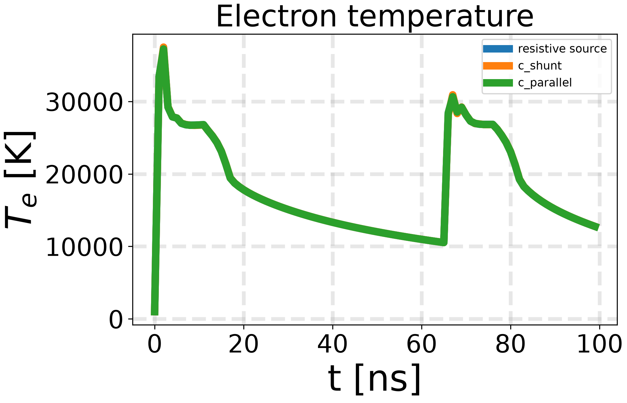
Case 1 (resistive source): completed, peak Te = 37236 K
Case 2: c_shunt – C_s shunts the source’s own output node to ground, in parallel with the cable’s input. Stateful (its own terminal voltage is an ODE solution), but – like TransmissionLineRCLoadCircuit in Tutorial 7 – called directly by the reactor: TransmissionLineCapacitiveSourceResistiveLoadCircuit wraps its own internal DrivenCircuitAdapter, so no external adapter is needed here. window_span is capped by the cable’s round trip (~65.3 ns) and chosen well below it for causality margin; net.max_time_step follows the usual window_span/2 bound.
shunt_source = CapacitiveSourceCircuit(
    TrapezoidalGenerator(U_on=U_ON, t_rise=T_RISE, t_on=T_ON, t_fall=T_FALL),
    R_g=R_G,
    C_s=C_S,
)
shunt_circuit = TransmissionLineCapacitiveSourceResistiveLoadCircuit(
    source=shunt_source,
    cable=CABLE,
    window_span=WINDOW_SPAN,
    include_reflections=True,
    r_p_rtol=R_P_RTOL,
)
reactor_shunt = _make_reactor(shunt_circuit)
net_shunt = ct.ReactorNet([reactor_shunt])
net_shunt.max_time_step = WINDOW_SPAN / 2

results_shunt = _run_case(reactor_shunt, net_shunt)
print(
    f"Case 2 (c_shunt source): completed, peak Te = {results_shunt['Te'].max():.0f} K"
)
Case 2 (c_shunt source): completed, peak Te = 37497 K
Case 3: c_parallel – the same C_s instead bridges R_g itself (a different node, a different ODE – see the module docstring). Same window_span/max_time_step reasoning as case 2.
parallel_source = ParallelCapacitiveSourceCircuit(
    TrapezoidalGenerator(U_on=U_ON, t_rise=T_RISE, t_on=T_ON, t_fall=T_FALL),
    R_g=R_G,
    C_s=C_S,
)
parallel_circuit = TransmissionLineParallelCapacitiveSourceResistiveLoadCircuit(
    source=parallel_source,
    cable=CABLE,
    window_span=WINDOW_SPAN,
    include_reflections=True,
    r_p_rtol=R_P_RTOL,
)
reactor_parallel = _make_reactor(parallel_circuit)
net_parallel = ct.ReactorNet([reactor_parallel])
net_parallel.max_time_step = WINDOW_SPAN / 2

results_parallel = _run_case(reactor_parallel, net_parallel)
print(
    "Case 3 (c_parallel source): completed, "
    f"peak Te = {results_parallel['Te'].max():.0f} K"
)
Case 3 (c_parallel source): completed, peak Te = 37240 K
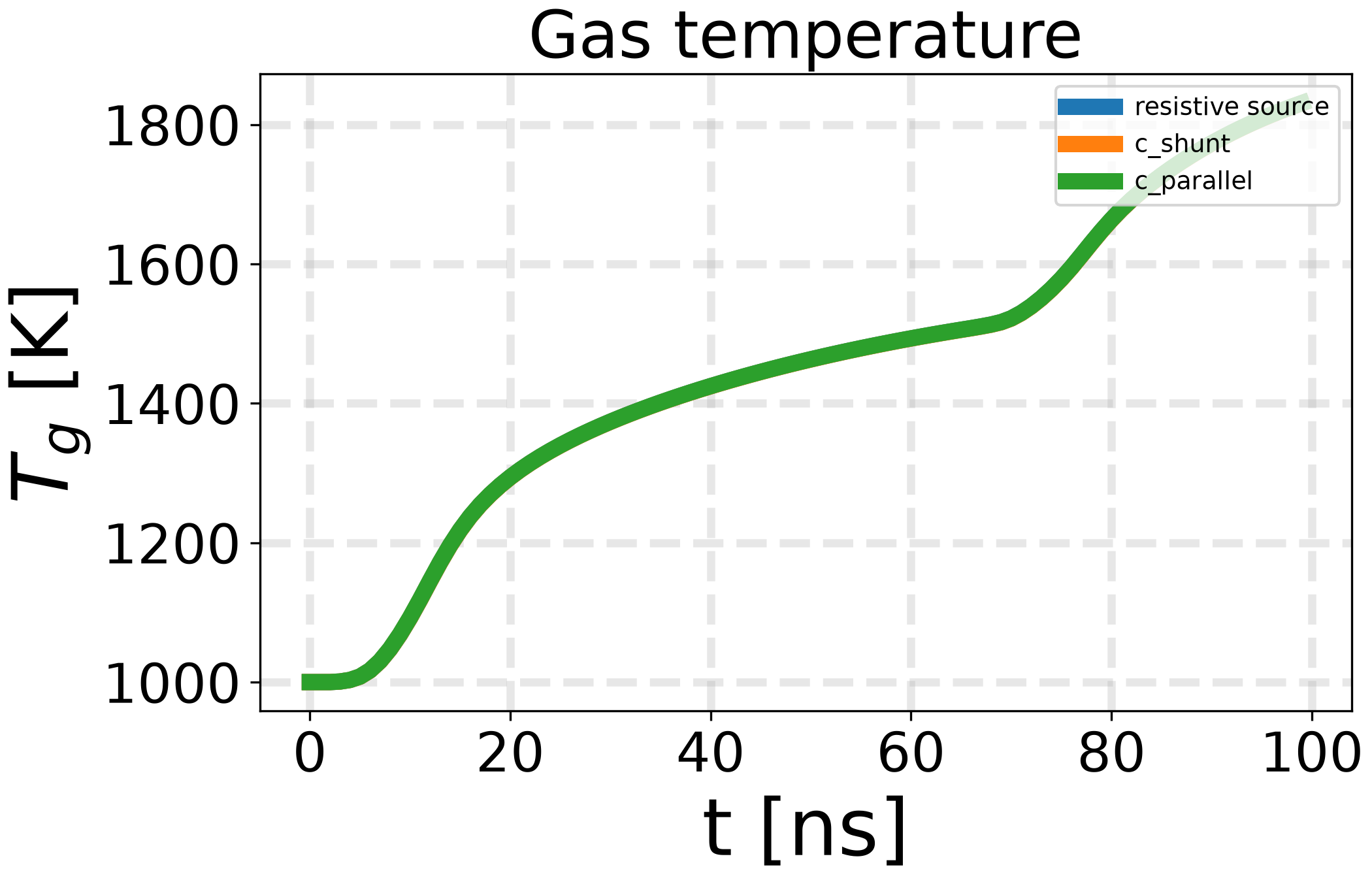
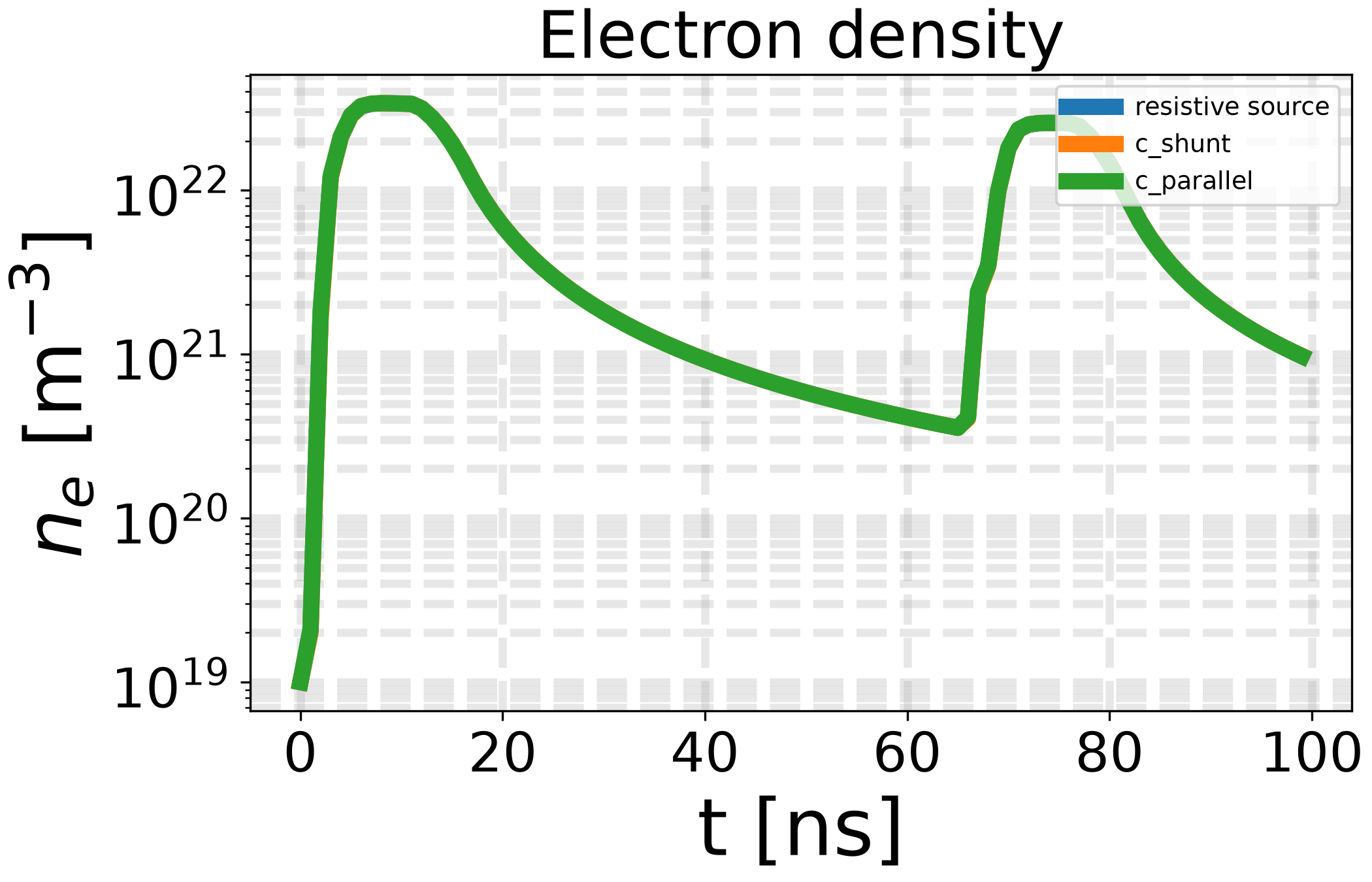
Compare all three cases across Te, Tg, ne, and Vp.
CASES = [
    ("resistive source", results_line),
    ("c_shunt", results_shunt),
    ("c_parallel", results_parallel),
]


def _compare_plot(key: str, y_label: str, title: str, log: bool = False) -> None:
    fig, ax = plt.subplots(figsize=(7, 4.5))
    for label, results in CASES:
        ax.plot(results["t"] * 1e9, results[key], label=label)
    ax.set_xlabel("t [ns]")
    ax.set_ylabel(y_label)
    ax.set_title(title)
    if log:
        ax.set_yscale("log")
    ax.legend(fontsize=9)
    ax.grid(alpha=0.3, which="both" if log else "major")
    plt.show()


_compare_plot("Vp", r"$V_p$ [V]", "Plasma voltage")
_compare_plot("Te", r"$T_e$ [K]", "Electron temperature")
_compare_plot("Tg", r"$T_g$ [K]", "Gas temperature")
_compare_plot("ne", r"$n_e$ [m$^{-3}$]", "Electron density", log=True)
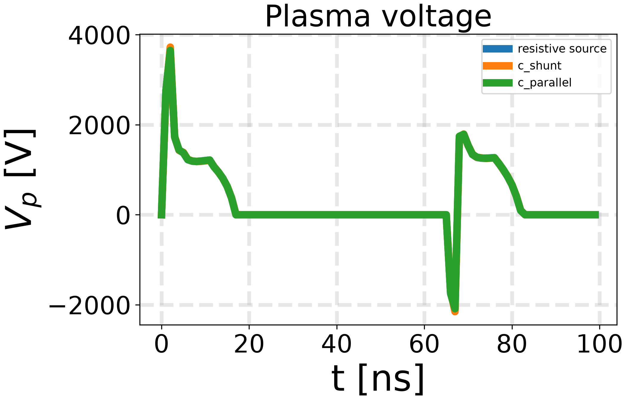
c_parallel’s much weaker forcing term (see module docstring) means its plasma voltage deviation from the resistive baseline sits ~30x smaller than c_shunt’s for this same C_s – invisible next to c_shunt on the shared-scale Vp plot above. Each deviation on its own, independently-scaled axis:
n = min(len(results_line["t"]), len(results_shunt["t"]), len(results_parallel["t"]))
t_ns = results_line["t"][:n] * 1e9
dVp_shunt = results_shunt["Vp"][:n] - results_line["Vp"][:n]
dVp_parallel = results_parallel["Vp"][:n] - results_line["Vp"][:n]
print(
    f"Peak |Vp deviation from resistive baseline|: "
    f"c_shunt = {np.max(np.abs(dVp_shunt)):.1f} V, "
    f"c_parallel = {np.max(np.abs(dVp_parallel)):.1f} V"
)

fig, (ax_shunt, ax_parallel) = plt.subplots(1, 2, figsize=(10, 4), sharex=True)
ax_shunt.plot(t_ns, dVp_shunt, color="tab:orange")
ax_shunt.set_title("c_shunt - resistive")
ax_parallel.plot(t_ns, dVp_parallel, color="tab:green")
ax_parallel.set_title("c_parallel - resistive")
for ax in (ax_shunt, ax_parallel):
    ax.set_xlabel("t [ns]")
    ax.set_ylabel(r"$\Delta V_p$ [V]")
    ax.grid(alpha=0.3)
fig.tight_layout()
plt.show()
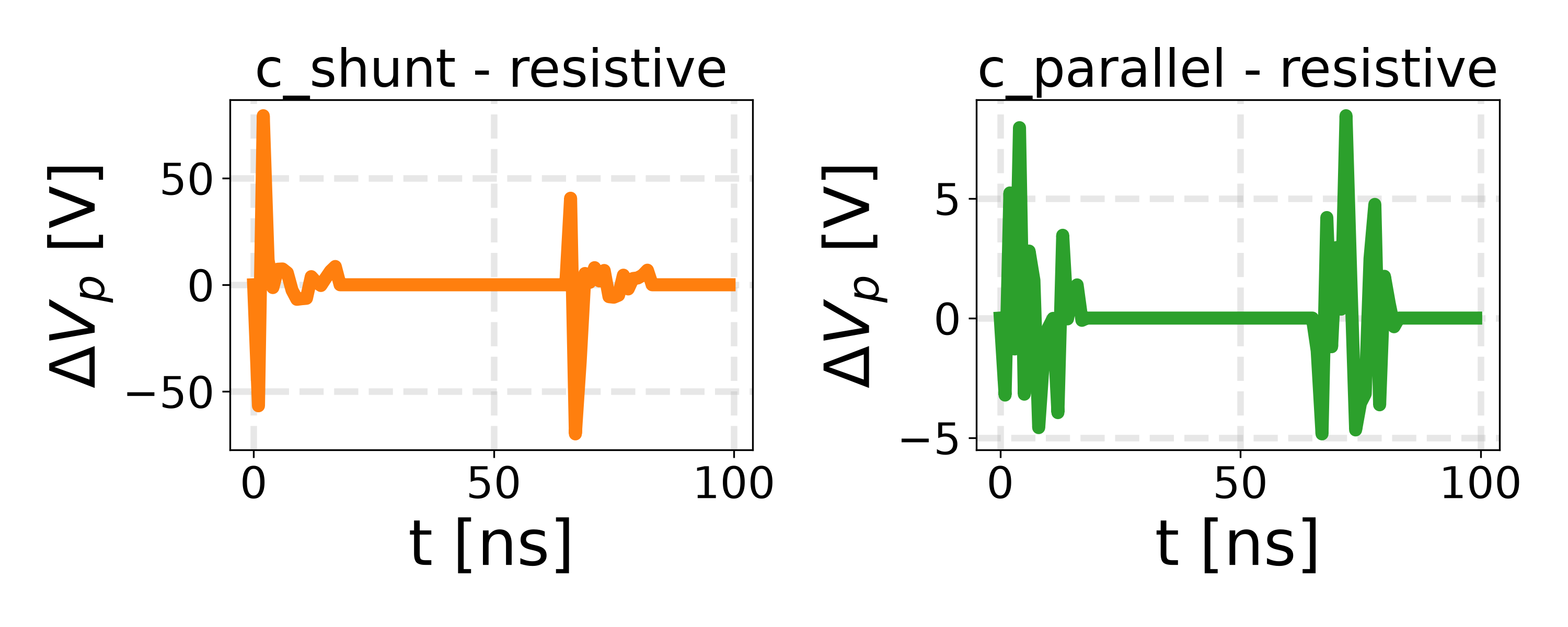
Peak |Vp deviation from resistive baseline|: c_shunt = 79.3 V, c_parallel = 8.5 V
/home/runner/work/rizer/rizer/examples/electric_circuit/plot_08_capacitive_source_circuit_comparison.py:300: UserWarning: The figure layout has changed to tight
  fig.tight_layout()
c_shunt rounds off the plasma voltage’s leading and trailing edges relative to the resistive baseline: the capacitor at the source’s own output node must charge through \(R_g \| Z_c\) before the launched wave tracks the generator’s own trapezoid. c_parallel bridges \(R_g\) itself instead – a different node, a different ODE, driven by a term ~:math:Z_c/R_g times weaker (module docstring) – so for the same \(C_s\) it produces a measurably smaller but still genuine perturbation, of a visibly different shape once viewed on its own scale. Both source networks converge to the same plateau, and to the resistive baseline, once the generator’s own voltage is flat; the downstream discharge (\(T_e\), \(T_g\), \(n_e\)) inherits each source’s own transient, most visibly during the rising edge.
Total running time of the script: (3 minutes 3.853 seconds)