Nanosecond pulse with a self-consistent circuit and radial hydrodynamics

ChannelReactor1D closes the NRP circuit on the channel’s own plasma resistance, \(R_p = \mathrm{gap} / \int \sigma \,\mathrm{d}A\), and – with hydrodynamics=True – advances continuity, radial momentum, species advection and the two pool energies alongside the chemistry. A broadening, rarefying channel therefore loads the line and pulls its own field down.

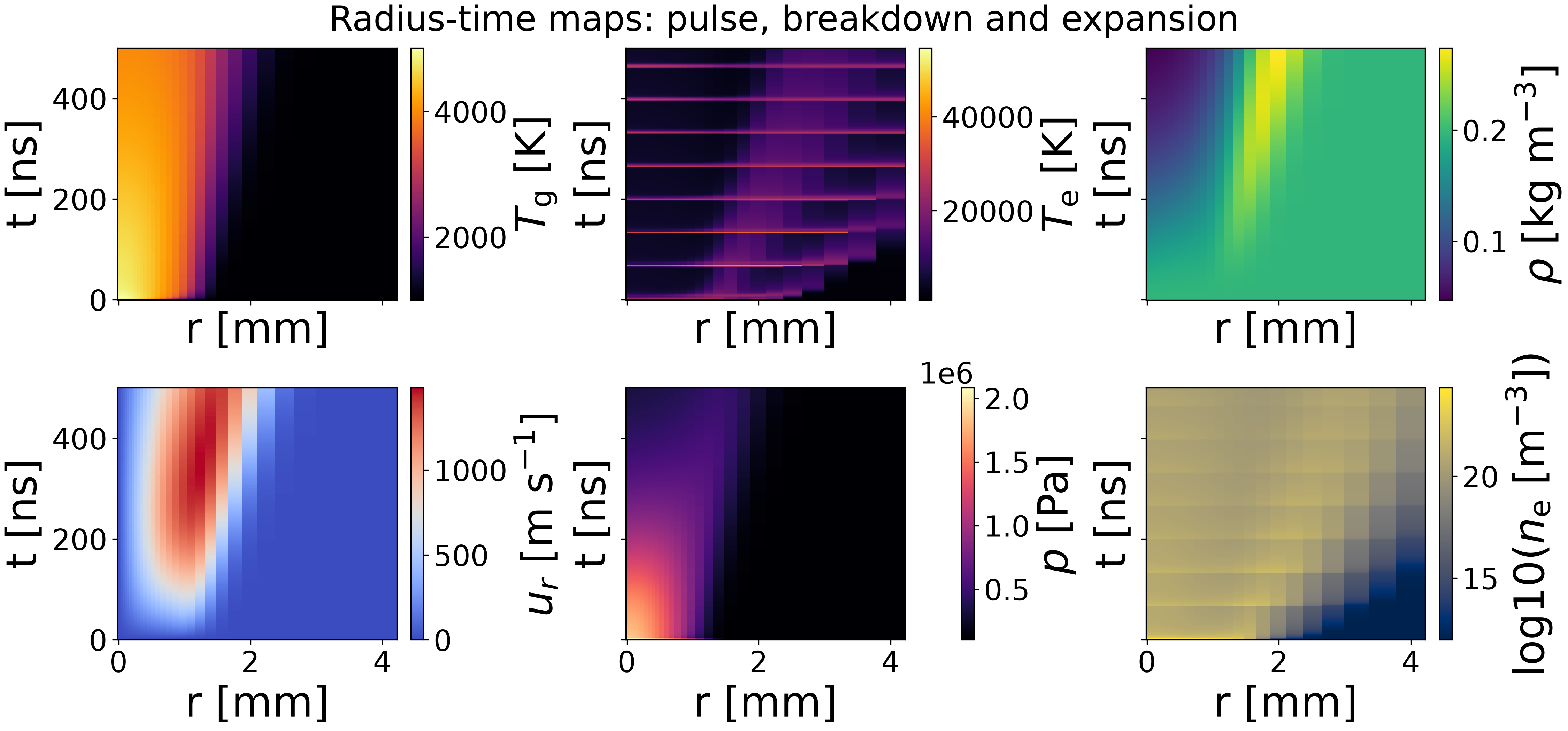
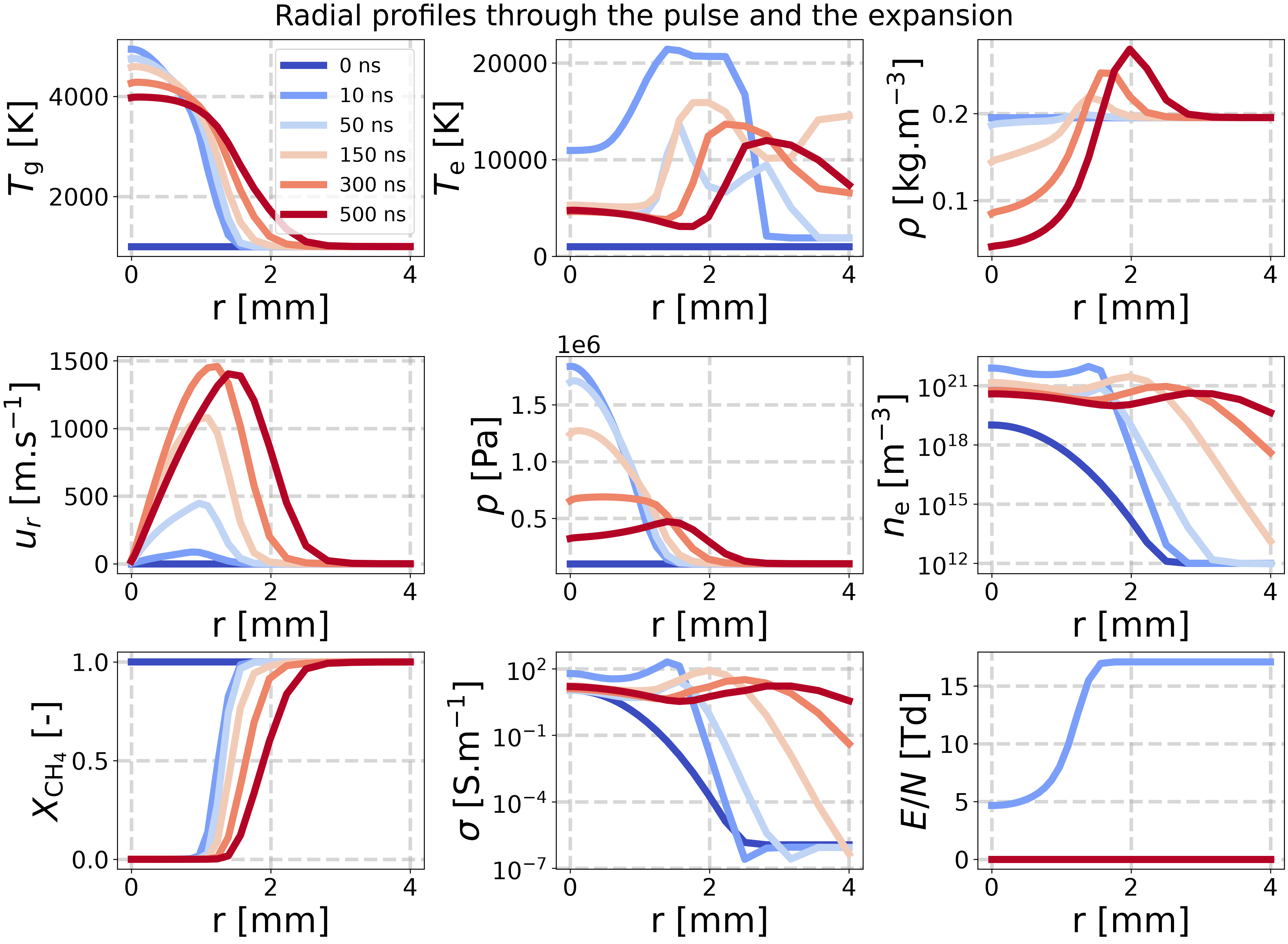
This example fires a 7 kV, roughly 12 ns trapezoidal pulse into a 3.8 mm gap of CH4 at atmospheric pressure and follows the channel for 500 ns. The discharge avalanches: \(T_e\) reaches 4.7 eV, \(n_e\) rises five decades, and \(R_p\) collapses from 298 to 0.05 ohm. The gas then expands at over a kilometre per second and the axis rarefies by three quarters – the mechanism a fixed-density channel model cannot represent at all.

Conduction and species diffusion are off (kappa = 0), so what is plotted is the pulse, the chemistry and the hydrodynamics alone.

Tags: plasma Cantera two-temperature transient channel hydrodynamics circuit NRP 1D

Import the required libraries.

import time

import cantera as ct
import matplotlib.pyplot as plt
import numpy as np

import rizer.kinetics.extensible_rate  # noqa: F401 (registers the CH4 rates)
import rizer.misc.units as u
from rizer.cantera_ext import _plasma1d
from rizer.electrical_model.circuit.transmission_line_circuit import (
    TransmissionLineResistiveCircuit,
)
from rizer.electrical_model.components.cable import IdealCable
from rizer.electrical_model.components.generator import TrapezoidalGenerator
from rizer.electrical_model.components.source_circuit import ResistiveSourceCircuit
from rizer.kinetics.electron_reactions import (
    electron_reaction_indices,
    species_formation_enthalpy_0K,
)
from rizer.misc.ct_utils import partially_ionized_mole_fractions
from rizer.misc.plt_utils import set_mpl_style
from rizer.misc.utils import get_path_to_data
from rizer.models.nrp.plasma_channel_split_2T1D import ChannelReactor1D
from rizer.transport.cpp_interop import unpack_momentum_transfer_models
from rizer.transport.loaders import get_default_momentum_transfer_collision_frequencies

set_mpl_style()

Discharge, circuit and grid.

The gap and cable follow plot_1d_vs_0d_selfconsistent.py; the generator is scaled to 7 kV over about 12 ns. The applied field is not U_on / gap: the circuit sets V_p against the channel’s own resistance, so a more conductive channel loads the line and lowers its own field.

mechanism = str(get_path_to_data("mechanisms") / "Goutier2025" / "CH4_to_C2H2.yaml")

gap = 3.8e-3  # Inter-electrode gap [m]
kernel_radius = 500e-6  # Seed ionization width (FWHM) [m]
r_wall = 4.0e-3  # Domain outer radius [m]

p_0 = ct.one_atm  # Initial pressure [Pa]
Tg_0 = 1000.0  # Initial gas and electron temperature [K]
ne_0 = 1.0e19  # Peak seed electron density [m^-3]

U_on = 7000.0  # Generator voltage when on [V]
t_rise, t_on, t_fall = 3e-9, 6e-9, 3e-9  # Trapezoid timings [s]

t_end = 500e-9  # End time [s]
dt_out = 1e-9  # Output cadence [s]
n_radial_points = 31  # Radial nodes [-]


def make_circuit():
    """Build the NRP circuit (trapezoidal generator + ideal cable)."""
    return TransmissionLineResistiveCircuit(
        source=ResistiveSourceCircuit(
            TrapezoidalGenerator(
                U_on=U_on, U_off=0.0, t_rise=t_rise, t_on=t_on, t_fall=t_fall
            ),
            R_g=1.0,
        ),
        cable=IdealCable(L=6.2, Z_c=75.0, c=1.9e8),
        include_reflections=True,
    )

Seed a Gaussian ionized core and run the channel.

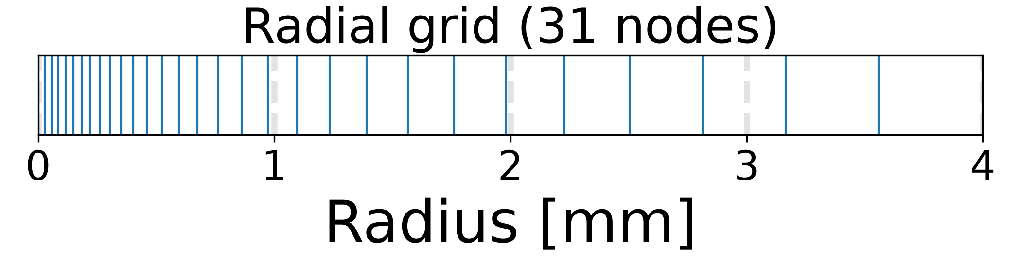
The grid is stretched toward the axis, where the gradients are. Y_amb is the ambient composition the outer ghost cell is held at; it is required once hydrodynamics is on, because the species fluxes only telescope into the mass flux at the wall when it sums to one.

plasma = ct.Solution(mechanism, "plasma", transport_model=None)
names = list(plasma.species_names)
mtcf = get_default_momentum_transfer_collision_frequencies(names)

r = r_wall * np.sinh(3.5 * np.linspace(0.0, 1.0, n_radial_points)) / np.sinh(3.5)
# Plot the radial grid
fig, ax = plt.subplots(figsize=(7.0, 1.8))
ax.vlines(r * 1e3, 0.0, 1.0, color="tab:blue", linewidth=1.0)
ax.set(
    xlabel="Radius [mm]",
    yticks=[],
    xlim=(0.0, r_wall * 1e3),
    ylim=(0.0, 1.0),
    title=f"Radial grid ({n_radial_points} nodes)",
)
ax.grid(axis="x", alpha=0.35)
plt.show()

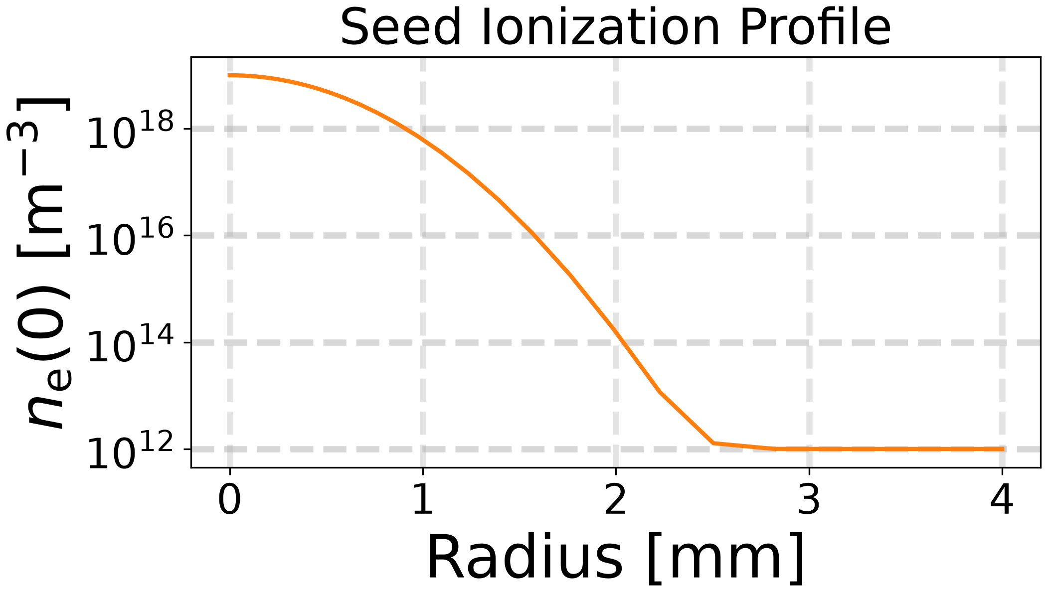
# Create and plot the initial electron density profile
width = kernel_radius / np.sqrt(2.0 * np.log(2.0))
ne_profile = ne_0 * np.exp(-(r**2) / (2.0 * width**2)) + 1.0e12
fig, ax = plt.subplots(figsize=(7.0, 4))
ax.plot(r * 1e3, ne_profile, color="tab:orange", linewidth=2.0)
ax.set(
    xlabel="Radius [mm]",
    ylabel=r"$n_\text{e}(0)$ [$\text{m}^{-3}$]",
    title="Seed Ionization Profile",
)
ax.set_yscale("log")
ax.grid(axis="x", alpha=0.35)
plt.show()

# Set the initial composition.
gas = ct.Solution(mechanism, "plasma")
Y0 = np.zeros((n_radial_points, plasma.n_species))
for node in range(n_radial_points):
    x_e = ne_profile[node] * u.k_b * Tg_0 / p_0
    X0 = partially_ionized_mole_fractions(x_e, background="CH4", ion="CH4+")
    gas.TPX = Tg_0, p_0, X0
    Y0[node] = gas.Y
# Set the ambient composition to CH4.
gas.TPX = Tg_0, p_0, "CH4:1"
Y_ambient = gas.Y.copy()

# Create the channel.
x_e = ne_0 * u.k_b * Tg_0 / p_0
X0 = partially_ionized_mole_fractions(x_e, background="CH4", ion="CH4+")
plasma.TPX = Tg_0, p_0, X0
channel = ChannelReactor1D(
    mech=mechanism,
    phase="plasma",
    grid=r,
    rho=float(plasma.density),
    mtcf=mtcf,
    species_names=names,
    reacting=True,
    kappa=0.0,
    T_amb=Tg_0,
    p_ext=p_0,
    hydrodynamics=True,
    Y_amb=Y_ambient,
    hydro_substep=None,
    outer_bc_mode="ambient_ghost",
)

t_out = np.arange(0.0, t_end + 1e-12, dt_out)
print("running the reacting hydrodynamic channel on its own circuit ...")
t_start = time.time()

# Solve channel with split circuit, which returns a history of the state variables.
history = channel.solve_split_circuit(
    t_out,
    make_circuit(),
    gap,
    np.full(n_radial_points, Tg_0),
    np.full(n_radial_points, Tg_0),
    Y0,
)
print(f"  done in {time.time() - t_start:.1f} s")

• 
• 

running the reacting hydrodynamic channel on its own circuit ...
  done in 81.1 s

Collect the history into arrays for plotting.

Tg = np.array(history["Tg"])
Te = np.array(history["Te"])
rho = np.array(history["rho"])
u_r = np.array(history["u_r"])
pressure = np.array(history["p"])
electron_density = np.array(history["ne"])

Rp = np.array(history["Rp"])
Vp = np.array(history["Vp"])
Ip = np.array(history["I"])

# Compute and store power and cumulative energy.
power = Vp * Ip
cumulated_energy = np.zeros_like(Vp, dtype=float)
for i in range(len(t_out)):
    cumulated_energy[i] = np.trapezoid(power[: i + 1], t_out[: i + 1])
# cumulated_energy = np.cumsum(Ip * Vp) * dt_out
deposited = float(np.trapezoid(Ip * Vp, t_out))
print(
    f"  peak |I| = {np.max(np.abs(history['I'])):.1f} A, "
    f"R_p {history['Rp'][0]:.1f} -> {min(history['Rp']):.3f} ohm, "
    f"electrical energy delivered = {deposited * 1e6:.3f} uJ"
)
print(
    f"  peak Te = {Te.max() * u.k_b / u.e:.2f} eV, peak n_e = {electron_density.max():.2e} m^-3, "
    f"peak |u_r| = {np.abs(u_r).max():.0f} m/s"
)

peak |I| = 184.1 A, R_p 298.1 -> 0.049 ohm, electrical energy delivered = 4780.791 uJ
peak Te = 4.71 eV, peak n_e = 2.21e+24 m^-3, peak |u_r| = 1485 m/s

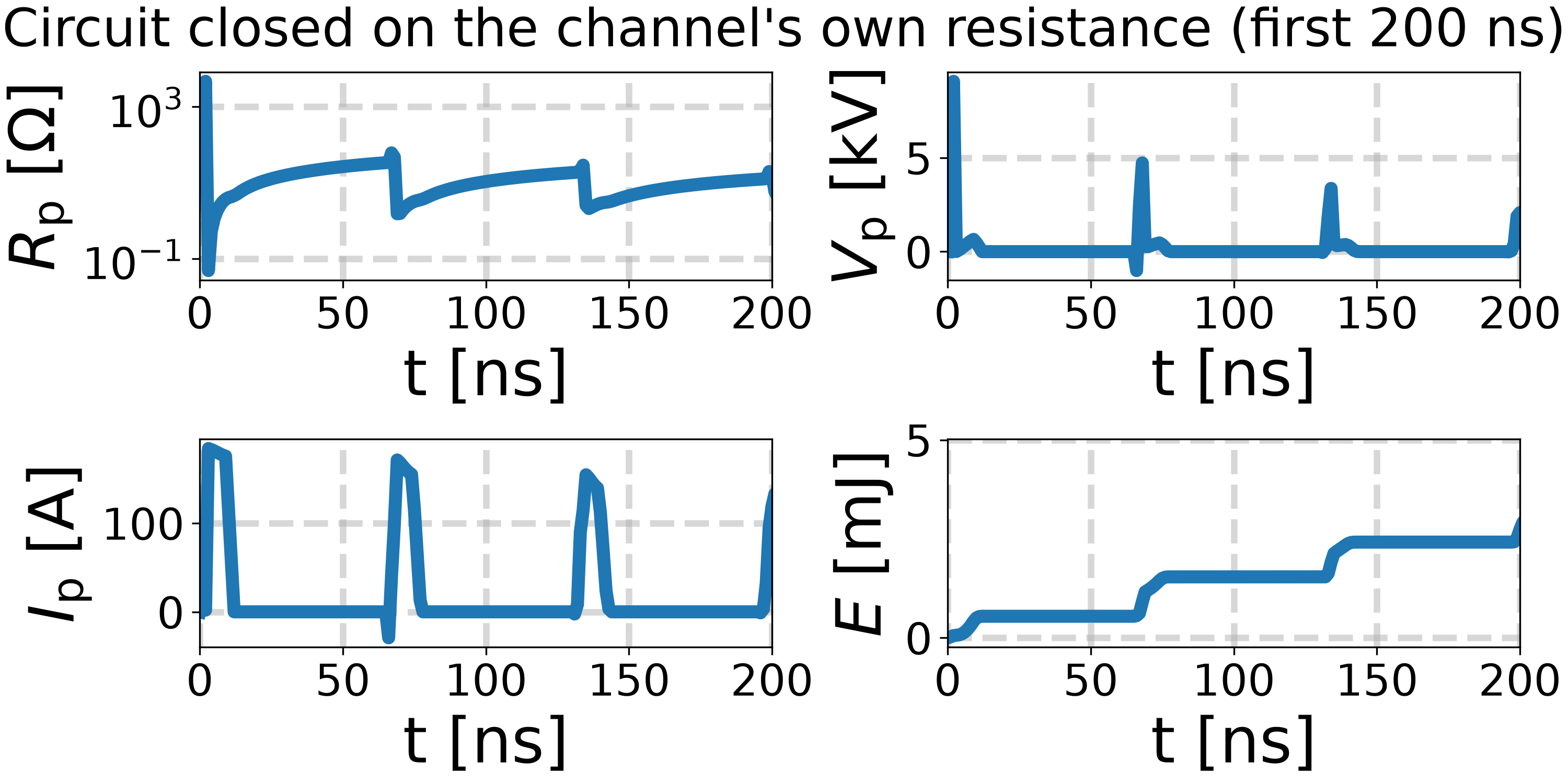
The circuit: the channel pulls its own field down.

R_p collapses as the gas ionizes, which loads the line; the late rise in V_p is the cable reflection returning after 2 L / c = 65 ns, long after the generator has finished.

fig, axes = plt.subplots(2, 2, figsize=(10, 5))
axes[0, 0].semilogy(t_out * 1e9, Rp)
axes[0, 0].set_ylabel(r"$R_\text{p}$ [$\Omega$]")
axes[0, 1].plot(t_out * 1e9, Vp * 1e-3)
axes[0, 1].set_ylabel(r"$V_\text{p}$ [kV]")
axes[1, 0].plot(t_out * 1e9, Ip)
axes[1, 0].set_ylabel(r"$I_\text{p}$ [A]")
axes[1, 1].plot(t_out * 1e9, cumulated_energy * 1e3)
axes[1, 1].set_ylabel(r"$E$ [mJ]")
for ax in axes.ravel():
    ax.set_xlabel("t [ns]")
    ax.set_xlim(0.0, 200.0)
fig.suptitle("Circuit closed on the channel's own resistance (first 200 ns)")

Text(0.5, 0.991666, "Circuit closed on the channel's own resistance (first 200 ns)")

Radius-time maps of the hydrodynamic state.

The pulse deposits its energy in the first few nanoseconds; the expansion that follows is what the hydro half-step adds. rho hollows out on the axis while u_r carries the gas outward.

r_mm, t_ns = r * 1e3, t_out * 1e9
fields = (
    (r"$T_\text{g}$ [K]", Tg, "inferno", False),
    (r"$T_\text{e}$ [K]", Te, "inferno", False),
    (r"$\rho$ [kg m$^{-3}$]", rho, "viridis", False),
    (r"$u_r$ [m s$^{-1}$]", u_r, "coolwarm", False),
    (r"$p$ [Pa]", pressure, "magma", False),
    (r"$n_\text{e}$ [m$^{-3}$]", electron_density, "cividis", True),
)
fig, axes = plt.subplots(2, 3, figsize=(15, 7), sharex=True, sharey=True)
for ax, (label, field, cmap, log) in zip(axes.ravel(), fields, strict=True):
    if log:
        field = np.log10(field)
        label = "log10(" + label + ")"
    mesh = ax.pcolormesh(r_mm, t_ns, field, shading="auto", cmap=cmap)
    fig.colorbar(mesh, ax=ax, label=label)
    ax.set_xlabel("r [mm]")
    ax.set_ylabel("t [ns]")
    ax.grid(None)
fig.suptitle("Radius-time maps: pulse, breakdown and expansion")

Text(0.5, 0.9940471428571429, 'Radius-time maps: pulse, breakdown and expansion')

Radial snapshots.

Overlaid profiles at a few representative times make the outward-running front and the hollowing axis explicit. The bottom row is what the chemistry and the circuit see: how much CH4 is left, the conductivity whose cross-section integral sets R_p, and the reduced field that drives the electron-impact rates.

snapshot_times = [0.0, 10e-9, 50e-9, 150e-9, 300e-9, t_end]
colors = plt.cm.coolwarm(np.linspace(0.0, 1.0, len(snapshot_times)))
snapshots = sorted(
    {min(int(round(t / dt_out)), len(t_out) - 1) for t in snapshot_times}
)

Y_hist = np.array(history["Y"])
E_applied = np.array(history["E"])

# Mole fractions and total number density straight from the mixture, rather
# than N = p / (k_B T): with two temperatures the pressure splits between the
# pools, so the ideal-gas form needs a temperature the mixture does not have.
moles_per_mass = Y_hist / plasma.molecular_weights  # [kmol/kg]
X = moles_per_mass / moles_per_mass.sum(axis=2, keepdims=True)
number_density = rho * moles_per_mass.sum(axis=2) * u.N_a_kmol  # [m^-3]
reduced_field = E_applied[:, None] / number_density / 1.0e-21  # [Td]

# Evaluated per snapshot off the frame's own density. `conductivity_profile`
# would read `channel.rho`, which the hydro step has since advanced to the
# final frame's.
conductivity = np.full_like(Tg, np.nan)
for frame in snapshots:
    conductivity[frame] = [
        channel.reactor.electrical_conductivity(
            Tg[frame, node],
            Te[frame, node],
            np.ascontiguousarray(Y_hist[frame, node]),
            rho[frame, node],
        )
        for node in range(n_radial_points)
    ]

profiles = (
    (r"$T_\text{g}$ [K]", Tg, False),
    (r"$T_\text{e}$ [K]", Te, False),
    (r"$\rho$ [kg.m$^{-3}$]", rho, False),
    (r"$u_r$ [m.s$^{-1}$]", u_r, False),
    (r"$p$ [Pa]", pressure, False),
    (r"$n_\text{e}$ [m$^{-3}$]", electron_density, True),
    (r"$X_{\text{CH}_4}$ [-]", X[:, :, names.index("CH4")], False),
    (r"$\sigma$ [S.m$^{-1}$]", conductivity, True),
    (r"$E/N$ [Td]", reduced_field, False),
)

fig, axes = plt.subplots(3, 3, figsize=(15, 11))
for ax, (label, field, log) in zip(axes.ravel(), profiles, strict=True):
    for frame, color in zip(snapshots, colors):
        ax.plot(r_mm, field[frame], label=f"{t_ns[frame]:.0f} ns", color=color)
    ax.set_xlabel("r [mm]")
    ax.set_ylabel(label)
    ax.set_yscale("log" if log else "linear")
axes[0, 0].legend(fontsize="small")
fig.suptitle("Radial profiles through the pulse and the expansion")

Text(0.5, 0.9962118181818181, 'Radial profiles through the pulse and the expansion')

The same discharge through the native solver.

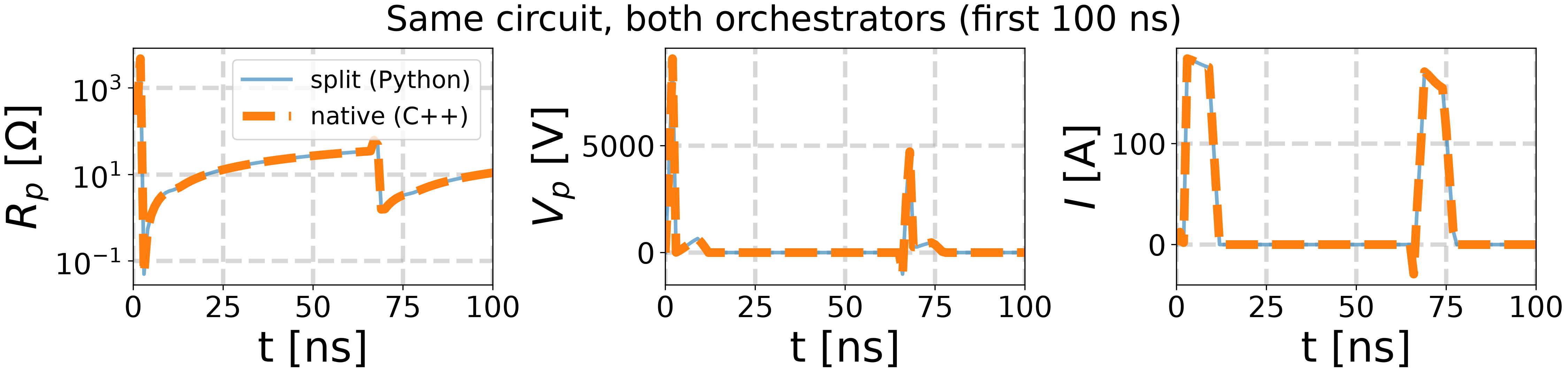
solve_1D_unsteady_discharge takes a plasma_voltage callback and closes the same circuit itself, exchanging two numbers per step: C++ hands out the channel’s resistance, Python returns the terminal voltage. The circuits are not ported – this is the same TransmissionLineResistiveCircuit object the split path used, driven from the other side.

independent_nodes is what makes it the faster path here: with kappa = 0 and no species diffusion the nodes are independent, so each gets its own integrator and its own step size instead of every node being advanced at the stiffest node’s pace.

Note the fresh circuit. The transmission line keeps a wave history, so a run must not inherit the previous one’s.

xsec_energy, xsec_sigma, radius_m, ion_charge = unpack_momentum_transfer_models(
    mtcf, plasma.n_species
)
native_circuit = make_circuit()

print("running the same case through the native solver ...")
t_start = time.time()
native = _plasma1d.solve_1D_unsteady_discharge(  # type: ignore
    mech=mechanism,
    phase="plasma",
    n_points=n_radial_points,
    R_max=r_wall,
    rho=float(plasma.density),
    Tg0=Tg_0,
    Te0=Tg_0,
    Y0=Y0[0],
    Y_amb=Y_ambient,
    sigma_T=None,
    sigma_v=None,
    nu_E=0.0,
    electric_field=0.0,
    kappa_H_T=None,
    kappa_H_v=None,
    kappa_e_T=None,
    kappa_e_v=None,
    D_species=0.0,
    reacting=True,
    T_amb=Tg_0,
    initTg_r=None,
    initTg_v=None,
    initTe_r=None,
    initTe_v=None,
    grid=r,
    nu_m=0.0,
    initY_r=r,
    initY_v=Y0,
    init_rho_r=None,
    init_rho_v=None,
    hydrodynamics=True,
    init_ur_r=None,
    init_ur_v=None,
    outer_bc_mode="ambient_ghost",
    p_amb=p_0,
    cfl=0.9,
    Efield_t=None,
    Efield_v=None,
    nu_m_T=None,
    nu_m_v=None,
    xsec_energy_J=xsec_energy,
    xsec_sigma_m2=xsec_sigma,
    radius_m=radius_m,
    ion_Z=ion_charge,
    Te_min=300.0,
    Te_max=1.0e5,
    Te_n=400,
    species_h0k=species_formation_enthalpy_0K(gas, electron_reaction_indices(gas)),
    dt=dt_out,
    n_steps=len(t_out) - 1,
    record_every=1,
    loglevel=0,
    rtol=1.0e-7,
    atol_T=1.0e-3,
    atol_Y=1.0e-9,
    independent_nodes=True,
    n_threads=1,
    gap=gap,
    plasma_voltage=lambda t, R_p: native_circuit.compute_plasma_voltage(t, R_p=R_p),
)
native_seconds = time.time() - t_start
print(f"  done in {native_seconds:.1f} s")

native_deposited = float(
    np.trapezoid(np.asarray(native["I"]) * np.asarray(native["Vp"]), t_out)
)
print(
    f"  peak |I| = {np.max(np.abs(native['I'])):.1f} A, "
    f"electrical energy delivered = {native_deposited * 1e6:.3f} uJ"
)

running the same case through the native solver ...
  done in 44.9 s
  peak |I| = 184.1 A, electrical energy delivered = 4779.750 uJ

The two paths agree, and the native one is faster.

They do not agree bit for bit and are not meant to: the reaction sub-step is per-node SciPy in one and CVODE in the other. What has to agree is the circuit the channel is loading, and it does.

fig, axes = plt.subplots(1, 3, figsize=(15, 3.6))
for ax, key, label in zip(
    axes,
    ("Rp", "Vp", "I"),
    (r"$R_p$ [$\Omega$]", r"$V_p$ [V]", r"$I$ [A]"),
    strict=True,
):
    ax.plot(t_ns, history[key], label="split (Python)", lw=2.5, alpha=0.6)
    ax.plot(t_ns, np.asarray(native[key]), label="native (C++)", ls="--")
    ax.set_xlabel("t [ns]")
    ax.set_ylabel(label)
    ax.set_xlim(0.0, 100.0)
axes[0].set_yscale("log")
axes[0].legend(fontsize="small")
fig.suptitle("Same circuit, both orchestrators (first 100 ns)")

plt.show()